GPD Parameter Stability#
Another popular graphical method to select the threshold when performing POT is the GPD Parameter Stability plots1. This technique is based on the property of GPD distribution of being “threshold stable”. This means that if the exceedances over a high threshold \(th_0\) follow a GPD with parameters \(\xi\) and \(\sigma_{th0}\), then for any other threshold \(th>th_0\), the exceedances will also follow a GPD with the same shape parameter \(\xi\) and a scale parameter \(\sigma_{th}=\sigma_{th0}+\xi(th-th_0)\).
Let \(\sigma^*=\sigma_{th}-\xi th\). Then, \(\sigma^*=\xi th_0\), which does not depend on \(th\) any more.
The parameter stability plot is then defined as
\( \{(th, \sigma^*); th<x_{max}\} \ and \ \{{(th, \xi); th<x_{max}}\} \)
where \(x_{max}\) is the maximum of the observations.
Therefore, \(\sigma^*\) and \(\xi_{th}\) are constant for all \(th>th_0\), if \(th_0\) is a suitable threshold for the asymptotic approximation. This is, the threshold should be chosen so the shape and scale parameters remain constant.
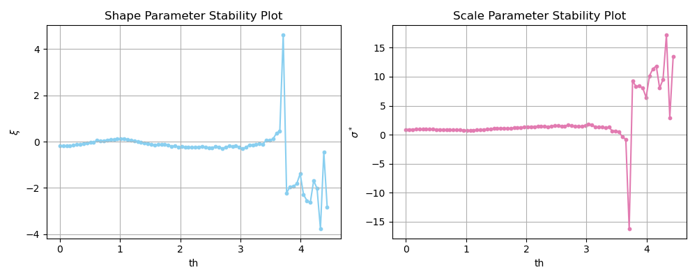
In summary, these plots present in the x-axis different values of \(th\) and in the y-axis the fitted \(\sigma^*\) or \(\xi\) for the values of \(th\) and a value of \(th\) where parameters remain stable should be selected. Note that this is also a graphical method and the interpretation of the analist has a role in the conclusions, being subjected to a certain degree of subjectivity.
In the figure below, you see an application of such method to our \(H_s\) data. We can see that both \(\xi\) and \(\sigma^*\) remain approximately stable for values \(th\leq 3.5m\). Thus, the previously selected \(th=2.5m\) is appropriate considering the Parameter Stability plots.
Let’s code it!#
In order to exemplify how to actually implement GPD Parameter Stability plots, pseudo code is presented. Note that here the first element in a vector corresponds to index 1.
read observations

#define parameters
dl = 48 #in hours
th = linspace(min_threshold, max_threshold, step) #range_thresholds

for i in length(th):
    excesses = find_peaks(observations, threshold = th[i], distance = dl) - th[i]
    scale[i], shape[i] = fit_GPD(excesses)
    modif_scale[i] = scale[1]-shape[i]*(th[i]-th[1])

plot(x = th, y = modif_scale)
plot(x = th, y = shape)
- 1
Coles (2004). An introduction to statistical modeling of extreme values. Sprinter-Verlang London.