Section 3: The Race between Slugs and Rabbits (trucks and cars!)#
NOTE: The last questions are extra material. Last year, this assignment was too long, but we didn’t want to remove it, as it may serve as a challenge for those of you that cover the material well. Besides, it is more practice material!
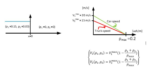
Now, we organize a multiclass traffic race. A platoon with \(20 %\) of trucks is waiting upstream at \(x = 0\) until the traffic signal turns green at \(t = 0\), see Figure 14 that represents the initial Riemann problem. We label the car flow as \(1\) with a density \(\rho_1\) and truck flow as \(2\) with a density \(\rho_2\). Figure 14 provides the fundamental diagrams in speed for both vehicle types and the model you should solve is given on slide 3 in the lecture 15.
The main objective is to draw the space-time diagram after the signal turns green. We are going to use two different methods. First, the linear approximation that allows you to make all calculations by yourself. However, it is clear here that the conditions for this approximation to be valid does not hold. Indeed, the jump in density between the left side (the platoon of vehicles) and the right side (void) is too high. By using then the full non-linear solution method, you will be able to assess the validity of the approximation.

Fig. 14 Initial traffic state and Fundamental diagrams in speed for each vehicle type#
Question 21#
Draw the state-space diagram using the linear approximation and determine the intermediate traffic states \(U_m\) at the front of the race.
Model Answer
Applying the linear approximation requires to define a steady state \(U_0\) along the full link. Indeed, the linear approximation is supposed to study the deviations \(\epsilon\) around this steady state (like the average water height and speed for the water flow). Here, the \(U_0\) is simply the average between the left (\(U_l\)) and the right (\(U_r\)) states.
The solution method for the linear approximation is given on slides 16, 17 and 18 of the lecture 15.
We need first to determine the common steady state \(U_0\) as the average of \(U_l\) and \(U_r\). Here, \(U_0\) is then equal to (\(\rho_1^0 = 0.075\); \(\rho_2^0 = 0.015\)). If we apply the multiclass model, we know that the elements of the \(\mathbf{A}\) matrix that defines the model is quasi linear form considering the given fundamental diagrams are:
We need to determine the two eigenvalues and the related eigenvectors for the state \(U_0\). The formulae are provided on slides 8 and 10 of lecture C4.1.c. The numerical results are \(\lambda_1 = 1.89 \mathrm{m/s}\); \(\lambda_2 = 8.7 \mathrm{m/s}\); \(w_1 = (4.65; 1)\); \(w_2 = (-1.43; 1)\)
To determine the intermediate state, one should first draw the line starting from \(U_l\) with a directed vector \(w_1\) and then draw the line starting from \(U_r\) with a directed vector \(w_2\). The intersection between these two lines give the intermediate state, here \(U_m = (0.0024, -0.0017)\).
Question 22#
Model Answer
The speed is equal to \(\lambda_2(U_0) = 8.7 \mathrm{m/s}\).
Question 23#
Model Answer
The intermediate state is not feasible because \(\rho_2^m <0 \). Also, the speed of the front wave looks way to slow compared to the maximal speed of the car that should be on the front of the race. The main reason is that the linear approximation does not hold. The jump in density between \(U_l\) and \(U_r\) is way too sharp.
Question 24#
Model Answer
By reading the state diagram, we see that \(U_m\) is \((0.0252, 5.74 \times 10^{-5})\). Now the intermediate state is feasible.
Question 25#
Model Answer
The front wave is rarefaction wave as the state diagram is composed of a 1-wave intersecting a 2-wave.
Model Answer
The wave speeds in the rarefaction wave are between \(\lambda_2(U_m)\) and \(\lambda_2(U_r) = 20 \mathrm{ m/s}\).
The maximal speed is then equal to \(20 \mathrm{ m/s}\) which represents the maximal speed of the cars.
Question 26#
Question 27#
Now, we change the right state to \((0.14, 0.02)\). The linear approximation should provide good results as the densities are close on both sides of the Riemann porblem. Calculate the intermediate state with the linear approximation. Then, use the python code to determine the intermediate state and compare the results.
Model Answer
With the linear approximation, \(U_m = (0.1321, 0.0276)\). The non-linear method gives \(U_m = (0.1323, 0.0272)\). The results are indeed very close and the linear approximation holds.
