11.5. Dutch rail level crossing#
Note
Press the rocket symbol on the top right of the page to make the page interactive and play with the code!
Problem statement#
Railways and roads often cross each other at evel-crossings. Because heavy vehicles must also be able to cross, the railway crossing is often cast in a concrete foundation. The mechanical properties of this concrete foundation are very different from the foundation of the other parts of the railway track. As a result, transitional radiation occurs during the passage of a train, potentially resulting in faster degradation of the local rail system or a negative passenger experience due to vibrational hindrance. Therefore, a transition zone is created by varying the number of sleepers and the distance between them to contribute to a smoother transition, which should have a positive effect on both operational performance and passenger comfort.
Step 1: Specify the design variables
In reality, this design depends on a multitude of design variables, but for now, it will be limited to just two of them:
\(F1 = x1 > 0\): the distance between the sleepers. Sleepers are the concrete (or sometimes wooden) beams that support the rails, as part of the ballast bed.
\(F2 = x2(≥ 1)\): the number of sleepers in the transition zone. The transition zone consists of a different type of sleeper than the rest of the track.
The key design performance functions describing the dynamic behaviour of the track at the level-crossing transition zone are the force \(F3 = F(x1, x2)\) and the acceleration \(F4 = a(x1, x2)\). These are usually the result of extensive numerical finite element and/or analytical calculations. For this design application, the physical/mechanical relationships between the design variables are simplified by using interpolation of discrete numerical calculations derived from a finite element based structural dynamic model (Shang et al., 2023). These interpolated results are the input to the design performance functions.
Step 2: Retrieve decision maker’s objectives
In this application several conflicting interests of multiple stakeholders are considered:
operational maintenance expenditures
travel comfort objective functions
capital investment
It is assumed that these three objectives are linked to three different stakeholders. Take for instance the Dutch ProRail organisation, where there is both a project delivery and a service operations department. They are linked to the capital and operational expenditure objectives, respectively. The Dutch train passenger is represented as the stakeholder linked to the travel comfort objective.
Step 3: Determine the preference functions for each objective
As mentioned before, three objective functions are investigated in this design application: maintenance costs, travel comfort and investment costs. Given these three objectives, the optimal design for the level-crossing zone is determined. The objective functions read as follows.
Maintenance costs (OPEX) are the key driver for the design of the level crossing transition zones. Large forces and accelerations will have a negative effect on the degradation of the track and foundations, resulting in increased maintenance costs. Hence, this objective can be written as a function of the force and acceleration. For that purpose, the force and acceleration are normalised and combined via the root sum of the square. The final maintenance costs per year objective reads as:
where
and where \(O_M\) expresses the OPEX per year in EUR. Note that at the level of design performance functions (i.e., apability-object level), it holds that \(F3 = F\) and \(F4 = a\) respectively.
Passenger travel comfort is an important consideration in railway design. When the dynamic behaviour (due to transition accelerations) during a passage of a level-crossing is substantial, it may lead to a negative travel experience or, in the worst case, to minor mishaps in the train (falling while walking, spilling drinks, etc.). To integrate this into the design problem, an objective is added that describes travel comfort as a function of the normalised acceleration:
Investment costs (CAPEX) must be considered as a key decision-making parameter. The installation of more sleepers will result in higher investment costs. However, more sleepers spread out over a greater distance will also mean that the investment costs for other parts of the rail will be reduced. Therefore, the investment costs objective can be represented as follows: $\(O_I = 1000 x_2 − 350 x_1 x_2\)\( where \)O_I$ expresses the CAPEX in EUR.
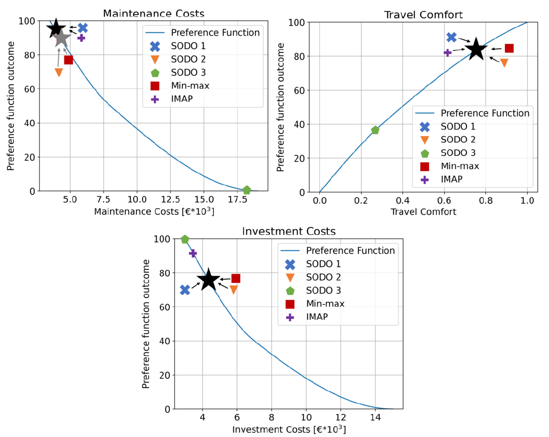
The preference functions for this design application are constructed based on the input from relevant stakeholders (Shang, 2021, 2023). The three resulting functions, which describe the relations between different values for P1..3,1..3 and O1..3, are shown as blue curves in the figure below (Figure 1). Note that the preference function elicitation was performed using the fundamentals of PFM research by (see Arkesteijn et.al. (2017)).
Step 4: To each objective assign decision maker’s weights
To generate the design points (i.e., design configuration results) for the different Multi-Objective Optimisation Methods (MODO Min-max and IMAP), the weights for each objective must first be determined. Since traditional (contractor) design offices often give a dominant weight to investment costs alone and less to the quality of service (QoS) oriented interests of maintenance and travel performance, here it is deliberately done ‘the other way round’, resulting in:
\(w_{1,M} = 0.4\) for maintenance
\(w_{2,C} = 0.4\) for travel comfort
\(w_{3,I} = 0.2\) for investments
For evaluation purposes, the design points for the different \(O_{(1...3)}\) Single-Objective Design Optimisations (SODO) are also determined for maintenance, investment costs and travel comfort respectively.
Step 5: Determine the design constraints
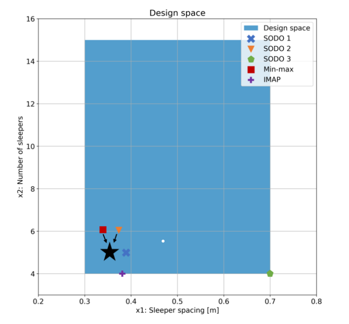
From the practical application context, the design variables are bounded by \(0.3 ≤ x1 ≤ 0.7\) and \(4 ≤ x2 ≤ 15\), which defines the design space (i.e., the solution space defined by the design variables (Figure 2)).
Step 6: Find the optimal design having the highest preference score
The outcomes of the different design points/configurations per optimisation method are first plotted in the preference functions showing the different objective values (\(O_{1..3}\)) and their corresponding individual preference values (\(P_{1..3,1..3}\)), respectively SODO 1, SODO 2 and SODO 3 in the legend (Figure 1).
Here below the results of the objective functions and the corresponding preference functions of the level-crossing design application:
Secondly, the numerical results of the different design points/configurations per optimisation method (SODO and/or MODO) can be read from the table below:
In this table one can find the aggregated preference score, which was used to determine the overall score/ranking via the PFM-based Multi-Criteria Decison Analysis (MCDA) tool Tetra (the resulting aggregated preference scores are rescaled between scores of 0 and 100, where 0 reflects the ‘worst’ scoring configuration/alternative and 100 the ‘best’ 1CITATION to APPENDIX )
Since there are only two design variables in this design application, we now plot the two-dimensional design space (sometimes referred to as solution space 1 ) containing the design points/configurations per optimisation method
The following three conclusions can be drawn from these figures and table:
The IMAP configuration is either equal to or closest to the best result on all single objectives (the SODO configurations). Only for the single-objective investment costs, IMAP is second best, since it also aims to optimise the other two objectives \(O_M\) and \(O_C\). For these objectives, a low sleeper spacing (\(x_1\)) is expected, while the number of sleepers (\(x_2\)) has a relatively small influence on the outcome of these objectives. For this design application in particular, and given the different objectives and associated stakeholder preferences, a low sleeper spacing (\(x_1\)) is expected to have a significant impact on objectives \(O_M\) and \(O_C\), while the number of sleepers (\(x_2\)) will have a smaller impact. However, for objective \(O_I\) , the influence of \(x_2\) will be significant, because for lower \(x_2\) the investment costs decreases. Furthermore, the influence of \(x_1\) on \(O_I\) is opposite to its influence on the other two objectives. Therefore, the design configuration that is optimised for investment costs only is not representative. A MODO optimisation is expected to find the ideal balance for the sleeper spacing (\(x_1\)), at lowest investment costs with the number of sleepers on the lower bound (i.e., \(x_2 = 4\)). The result of the IMAP optimisation does indeed reflect this best fit-for-common-purpose balance. As a result, IMAP may be characterised as a pure synthesis multi-objective design method.
The IMAP configuration achieves better or equal individual preference function values (\(P_{1..3,1..3}\)) and, more importantly, much better overall scores than the MODO min-max method result. This is because, according to the Min-max principle, this method will not be able to outperform the one objective score that shows the maximum attainable minimum distance to \(100\) (i.e., the minimum dissatisfaction). Thus, the min-max method inherently produces a sub-optimal compromise design configuration which, depending on the specific input parameters, can at best perform as well as the synthesis IMAP method. This limits the applicability of the Min-max method as a real multi-objective design optimisation method.
From the design space figure it is seen that, perhaps counter-intuitively, both the SODO 1 and 2 and the MODO min-max results fall within the design space (\(x_1\); \(x_2\) equals \(0.35/0.39\) and \(5\) respectively) and that the MODO IMAP and SODO 3 results lie on the edge and in a corner point of the design space respectively. This is because the set of design points that fall within the design space are the result of optimising the ’technical’ design performance only. In other words, this means that these optimal solutions move to an optimum only within the feasibility space (i.e., a solution space defined by the physical engineering variables only, and which is a subset of the design space) and lie on the ’classical’ Pareto front. Note that in this case a possible Pareto front, which defines an edge of the feasibility space as a function of \(F\) and \(a\), results only from the minimisation of \(O_M\) and \(O_C\). Despite the fact that SODO 3 actually does find the edges of the design space (corner point), it still scores low overall because it is by far the lowest on the other two objectives (1 and 2). MODO IMAP gives the overall best design point on the edge of the design space (\(x_1\) and/or \(x_2\) equals \(0.38\) and/or \(4\) respectively), and can therefore be considered the pure best fit-for-common-purpose design point.
Note that when the emphasis in the design application is on optimising the integrated socio-technical problem, the overall best configuration will be found within and/or on the edge of the design space. When optimising solely on cost or technics, one can either end up at the classical Pareto front or in a corner point of the design space


