8.5. Single-Objective Optimisation (SODO): Bridge Design Problem#
Note
Press the rocket symbol on the top right of the page to make the page interactive and play with the code!
In some cases, engineering design problems are simplified to a single-objective optimisation (SODO). This means that all weights are set to zero except for one objective, effectively focusing the analysis on just one stakeholder’s interest. While such simplifications can be useful as a first step, they should be understood as special cases of multi-objective optimisation (MODO).
Problem statement#
To illustrate, consider a bridge design where we limit the design problem to the determination of the optimal span and the clearance height of the bridge. Assume that there are two decision makers (stakeholders) that have conflicting interests:
The municipality, interested in the costs of the bridge.
The waterway users, interested in the waiting time when the bridge is closed for waterway users.
Step 1: Specify the design variables
For this problem we have two controllable design variables:
\(x_1\): the bridge span, and
\(x_2\): the clearance height of the bridge.
Step 2: Retrieve decision maker’s objectives
The municipality wants the cost to be minimised which becomes the first objective function \(O_1\), whereas the waterway users want the waiting time to be minimised which becomes the second objective function \(O_2\).
Step 3: Determine the preference functions for each objective
The costs are a function of the material use which in turn is a function of both the span and clearance height. We assume a linear relationship between costs \(O_1\) and material use \(F_1\) defined by coefficient \(c_1 = 3\).
We also assume a linear relationship between material use and both span and clearance height defined by coefficients \(c_2 = 4\) and \(c_3 = 7\) respectively.
The first objective to be minimised then becomes:
The waiting time is a function of the traffic flow which in turn is a function of both the span and clearance height. We again assume a linear relationship between waiting time \(O_2\) and traffic flow \(F_2\), and reads as:
where \(w_0 > 0\).
We also assume: (a) the coefficient \(c_4 = 1.2\); (b) a maximal waiting time of \(w_0 = 100\) (for a traffic flow that is ’nearly’ zero); (c) a linear relationship between traffic flow and both span and clearance height defined by coefficients \(c_5 = 1.7\) and \(c_6 = 1.9\) respectively.
The second objective to be minimised then becomes:
Step 4: To each objective assign decision maker’s weights
For this problem the weights are assumed to be equal, i.e. \(w_1 = w_2 = 0.5\).
Step 5: Determine the design constraints
The constraints relate to the minimum and maximum span and the minimum and and maximum clearance height:
Step 6: Find the optimal design having the highest preference score
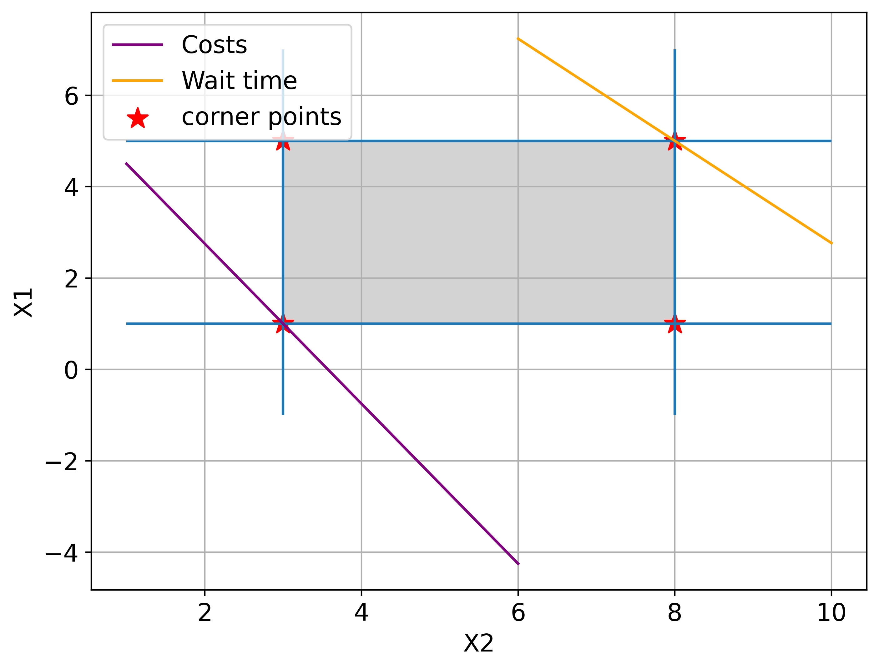
The graphical representation of this problem and both optimal solutions are shown in the figure below. Optimisation is carried out using MILP and Scipy Minimize. The design points are \((x1, x2) = (1, 3)\) and \((5, 8)\) for costs and waiting time respectively.
Therefor the
costs are minimised at \((x1, x2) = (1, 3)\), and
waiting time is minimised at \((x1, x2) = (5, 8)\).

Graphical representation of the bridge design problem.
The graphical results show that SODO produces different optima depending on the selected objective.
Python code for bridge design problem#
Type of algorithm used for single objective optimisation: Scipy minimize and MILP
Type of algorithm used for multi objective optimisation: Genetic Algorithm (tetra)
Number of design variables: 2
Number of objective functions: 2
Bounds: yes
Constraints: no
Type of problem: linear
# ==== SAFE MATPLOTLIB BOOTSTRAP (run this cell first) ====
import os, sys, importlib

def _in_ipython_kernel():
    try:
        from IPython import get_ipython
        ip = get_ipython()
        return bool(ip) and hasattr(ip, "kernel")
    except Exception:
        return False

import matplotlib
_backend_set = False

if _in_ipython_kernel():

    try:
        importlib.import_module("matplotlib_inline.backend_inline")
        matplotlib.use("module://matplotlib_inline.backend_inline", force=True)
        _backend_set = True
    except Exception as e:
        print("[warn] inline backend niet beschikbaar/compatibel:", e)

if not _backend_set:

    try:
        matplotlib.use("Agg", force=True)
        print("[info] Using Agg backend (no GUI).")
    except Exception as e:
        print("[warn] Agg backend kon niet gezet worden:", e)

import matplotlib.pyplot as plt

try:
    from IPython.display import display, Image
    def _safe_show():
        import uuid
        fname = f"_plot_{uuid.uuid4().hex}.png"
        plt.savefig(fname, bbox_inches="tight")
        display(Image(filename=fname))
        plt.close('all')
    if matplotlib.get_backend().lower() == "agg":
        plt.show = _safe_show
except Exception:
    # No IPython: show will not work
    pass

# Optionial, defaults
import matplotlib as mpl
mpl.rcParams.update({
    "figure.dpi": 100,
    "savefig.dpi": 120,
    "figure.figsize": (10, 5),
})

# Imports
import sys
import matplotlib.pyplot as plt
import numpy as np
from scipy.interpolate import pchip_interpolate
from scipy.optimize import minimize, LinearConstraint, milp
from matplotlib.patches import Polygon

from genetic_algorithm_pfm import GeneticAlgorithm
MILP and Minimise#
Scipy has two algorithms that can easily be used for optimisation: MILP and Minimize. The former is especially useful for mixed-integer problems: problems where one or more of the variables is an integer variable. The latter is, however, more straightforward in its use.
To show their applicability, the same problem is worked out with both methods in this notebook.
# define constants
c1 = 3   # costs per material
c2 = 4   # material used per metre bridge span
c3 = 7   # material used per metre air draft
c4 = 1.2   # relation between waiting time and traffic flow
c5 = 1.7   # traffic flow per metre bridge span
c6 = 1.9   # traffic flow per metre air draft

WT0 = 100   # minimal waiting time
MILP#
# first, define the objective function. Since it is linear, we can just provide the coefficients with which x1 and x2
# are multiplied. Note the -1: we need to maximize, however, milp is a minimization algorithm!
c_costs = 1 * np.array([c1 * c2, c1 * c3])
c_wait_time = -1 * np.array([c4 * c5, c4 * c6])

# next, define the constraints. For this we first provide a matrix A with all the coefficients x1 and x2 are multiplied.
A = np.array([[1, 0], [0, 1]])

# next we determine the upper bounds as vectors
b_u = np.array([5, 8])

# finally, we need to define the lower bound. In our case, these are taken as 0
b_l = np.array([1, 3])

# we can now define the LinearConstraint
constraints = LinearConstraint(A, b_l, b_u)

# the integrality array will tell the algorithm what type of variables (0 = continuous; 1 = integer) there are
integrality = np.zeros_like(c_costs)

# Run the optimization
result1 = milp(c=c_costs, constraints=constraints, integrality=integrality)
result2 = milp(c=c_wait_time, constraints=constraints, integrality=integrality)

print('Results MILP')
print(f'Objective 1 is minimal for x1 = {result1.x[0]} and x2 = {result1.x[1]}. The costs are then {result1.fun}.')
print(f'Objective 2 is minimal for x1 = {result2.x[0]} and x2 = {result2.x[1]}. '
      f'The wait time is then {result2.fun + WT0}.')
Results MILP
Objective 1 is minimal for x1 = 1.0 and x2 = 3.0. The costs are then 75.0.
Objective 2 is minimal for x1 = 5.0 and x2 = 8.0. The wait time is then 71.56.
Minimize#
# define objectives
def objective_costs(x):
    x1, x2 = x

    F1 = c2 * x1 + c3 * x2

    return c1 * F1


def objective_wait_time(x):
    x1, x2 = x

    F2 = c5 * x1 + c6 * x2

    return -1 * c4 * F2 + WT0


# define bounds for two variables
bounds = ((1, 5), (3, 8))

# initiate optimization
result1 = minimize(objective_costs, x0=np.array([1, 1]), bounds=bounds)
result2 = minimize(objective_wait_time, x0=np.array([1, 1]), bounds=bounds)

optimal_result_O1 = result1.fun
optimal_result_O2 = result2.fun

# print results
print('Results Minimize')
print(f'Objective 1 is minimal for x1 = {result1.x[0]} and x2 = {result1.x[1]}. The costs are then {result1.fun}.')
print(f'Objective 2 is minimal for x1 = {result2.x[0]} and x2 = {result2.x[1]}. The wait time is then {result2.fun}.')
print()
Results Minimize
Objective 1 is minimal for x1 = 1.0 and x2 = 3.0. The costs are then 75.0.
Objective 2 is minimal for x1 = 5.0 and x2 = 8.0. The wait time is then 71.56.
Plot the results#
After optimising using the minimise algorithm the solution space and the objective function are plotted.
# plot graphical solution
fig, ax = plt.subplots(figsize=(8, 6))

# Draw constraint lines
ax.vlines(3, -1, 7)
ax.vlines(8, -1, 7)
ax.hlines(1, 1, 10)
ax.hlines(5, 1, 10)

# Draw the feasible region
feasible_set = Polygon(np.array([[3, 1],
                                 [8, 1],
                                 [8, 5],
                                 [3, 5]]),
                       color="lightgrey")
ax.add_patch(feasible_set)

ax.set_xlabel('X2')
ax.set_ylabel('X1')

# Draw the objective function
x2 = np.linspace(1, 6)
ax.plot(x2, (optimal_result_O1 - c1 * c3 * x2) / (c1 * c2), color="purple", label='Costs')
x2 = np.linspace(6, 10)
ax.plot(x2, (WT0 - c4 * c6 * x2 - optimal_result_O2) / (c4 * c5), color="orange", label='Wait time')

ax.scatter([3,3,8,8], [1,5,1,5], marker='*', color='red', label='corner points', s=150)

ax.legend()
ax.grid()
plt.show();