8.6. Multi-Objective Optimisation (MODO): Bridge Design Problem#
Note
Press the rocket symbol on the top right of the page to make the page interactive and play with the code!
In reality, engineering design almost always involves multiple stakeholders with conflicting objectives. Therefore, multi-objective optimisation (MODO) is the more general and fundamental approach in preference-based engineering design.
SODO can be seen as a special case of MODO, obtained by assigning all weight to a single objective.
The bridge design problem is extended here to illustrate MODO. Instead of optimising each stakeholder’s objective separately, we evaluate trade-offs and find compromise solutions.
A priori optimisation
The single-objective optimisation in Section 8.5 considered each stakeholder separately and evaluated only the corner points of the design space. However, this is no guarantee that the true optimal solution is found. In fact, for the bridge design problem the optimal solution is not located at any of the corners.
This illustrates that single-objective optimisation is only a stepping stone. To identify true compromise solutions between conflicting objectives, a full multi-objective optimisation is required.
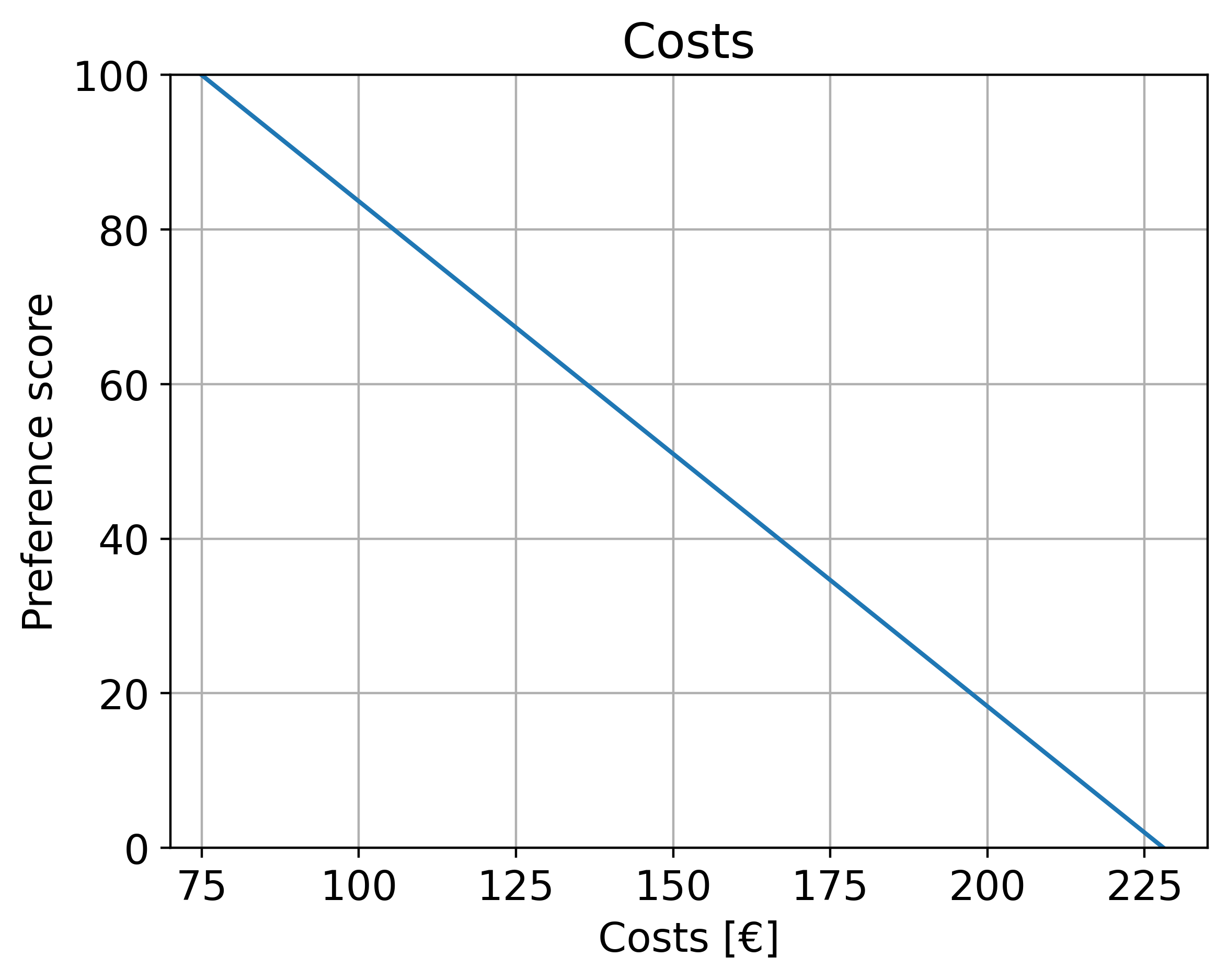
Step 1: Define the preference functions
For each stakeholder, we define preference functions that map objective values to preference scores.
Municipality (costs): preference decreases linearly with increasing construction costs.
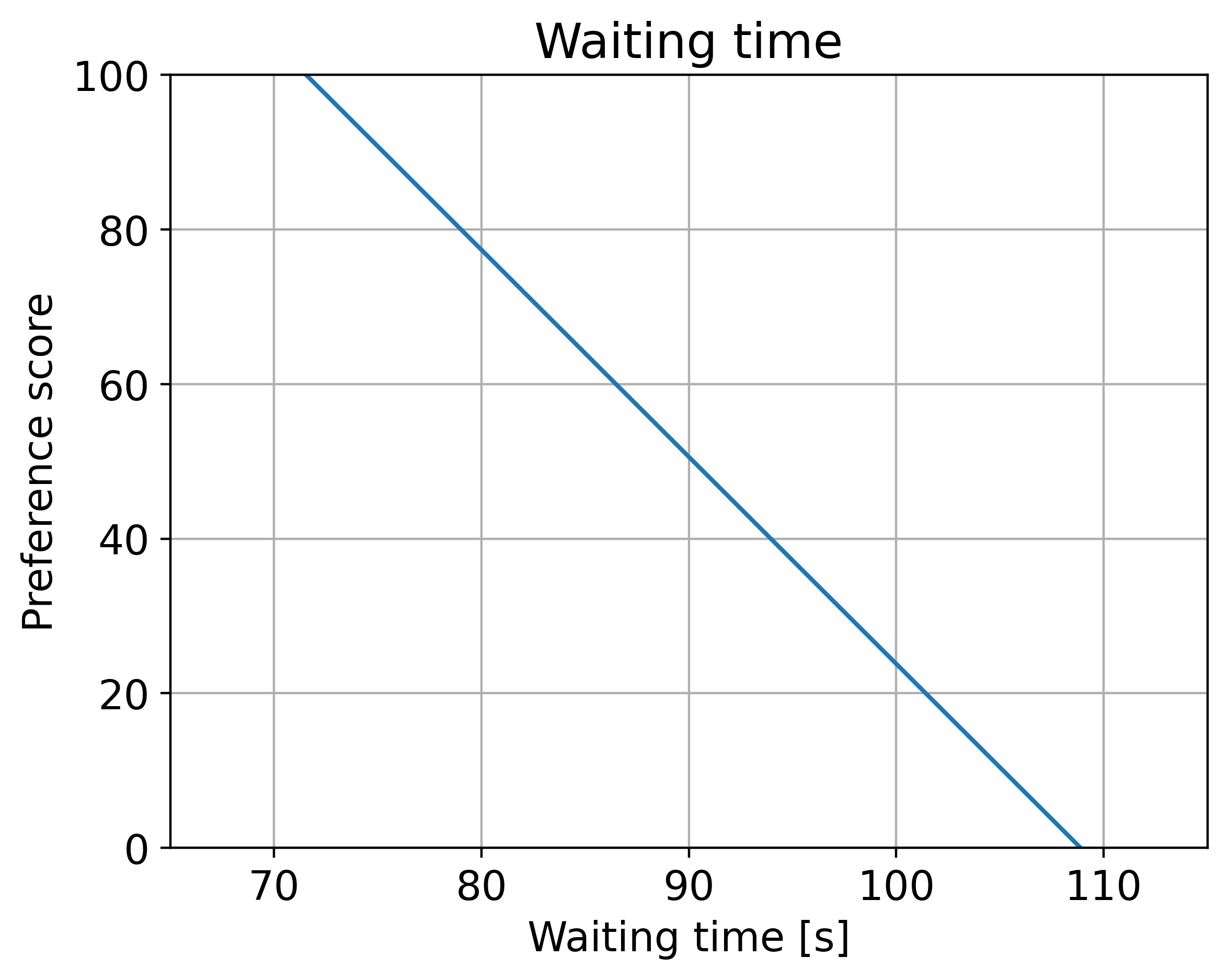
Waterway users (waiting time): preference decreases with increasing waiting time.
For example, costs of 75 yield a relatively high preference, whereas costs of 228 result in a very low preference. Similarly, waiting times near 71 seconds are rated highly, whereas values above 108 seconds are strongly penalised.
Step 2: Aggregate stakeholder preferences
To combine stakeholder preferences into a single evaluation, we use an aggregation method. Here, the a-fine aggregator is applied with equal weights for both stakeholders:
\(𝑤1= 𝑤2 = 0.5\)
This reflects the assumption that both the municipality and waterway users have equal influence in the decision-making process.
Step 3: Corner point evaluation
Before running a full optimisation, the feasible set’s corner points can be evaluated. This illustrates how preferences trade off against each other:
\(x_1\) |
\(x_2\) |
Aggregated preference |
|---|---|---|
1.0 |
3.0 |
36.68 |
1.0 |
8.0 |
0.00 |
5.0 |
3.0 |
100.00 |
5.0 |
8.0 |
63.32 |
These results already show that compromise solutions may exist, but again, optimality is not guaranteed at corners.
Step 4: Multi-objective optimisation with a Genetic Algorithm
To find the true optimal solution, a Genetic Algorithm (GA) is applied over the full design space. This algorithm searches iteratively for design solutions that maximise the aggregated preference score.
Parameters used:
Aggregation: a-fine
Population size: 120
Iterations: 1000 (stopping earlier if no improvement)
Crossover rate: 0.9
Variables: 𝑥1 (span) and 𝑥2 (clearance height)
The GA result for the bridge problem is:
\(𝑥1 ≈ 4.98\), \(𝑥2 ≈ 3.02\)
This solution balances both cost and waiting time, achieving a higher aggregated preference than the single-objective results.
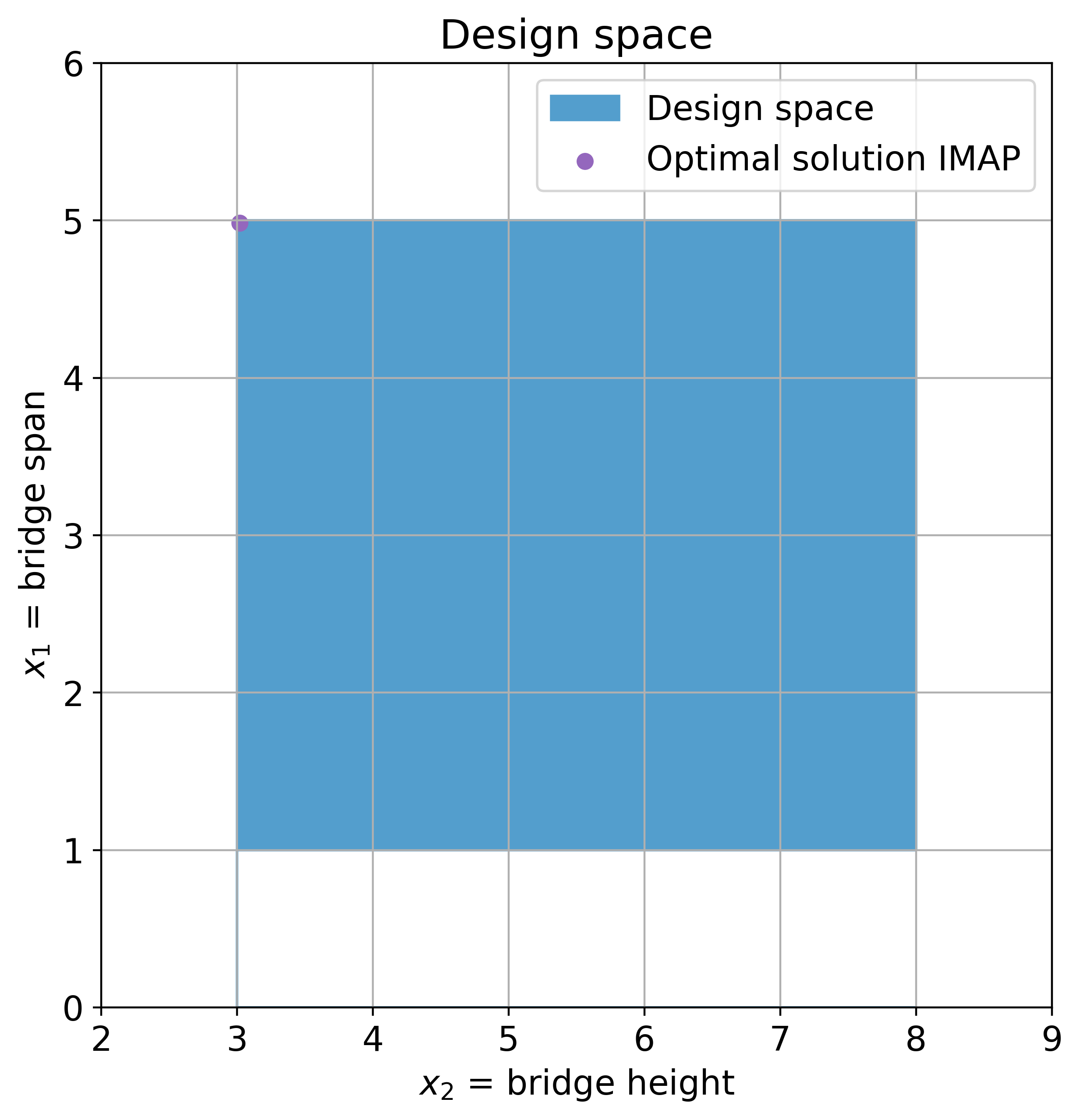
Step 5: Visualisation of results
The figure below shows the design space, the feasible region, and the optimal compromise solution identified by the GA.
Python code for bridge design problem#
Type of algorithm used for single objective optimisation: Scipy minimize and MILP
Type of algorithm used for multi objective optimisation: Genetic Algorithm (tetra)
Number of design variables: 2
Number of objective functions: 2
Bounds: yes
Constraints: no
Type of problem: linear
# ==== SAFE MATPLOTLIB BOOTSTRAP (run this cell first) ====
import os, sys, importlib

def _in_ipython_kernel():
    try:
        from IPython import get_ipython
        ip = get_ipython()
        return bool(ip) and hasattr(ip, "kernel")
    except Exception:
        return False

import matplotlib
_backend_set = False

if _in_ipython_kernel():

    try:
        importlib.import_module("matplotlib_inline.backend_inline")
        matplotlib.use("module://matplotlib_inline.backend_inline", force=True)
        _backend_set = True
    except Exception as e:
        print("[warn] inline backend niet beschikbaar/compatibel:", e)

if not _backend_set:

    try:
        matplotlib.use("Agg", force=True)
        print("[info] Using Agg backend (no GUI).")
    except Exception as e:
        print("[warn] Agg backend kon niet gezet worden:", e)

import matplotlib.pyplot as plt

try:
    from IPython.display import display, Image
    def _safe_show():
        import uuid
        fname = f"_plot_{uuid.uuid4().hex}.png"
        plt.savefig(fname, bbox_inches="tight")
        display(Image(filename=fname))
        plt.close('all')
    if matplotlib.get_backend().lower() == "agg":
        plt.show = _safe_show
except Exception:
    # No IPython: show will not work
    pass

# Optionial, defaults
import matplotlib as mpl
mpl.rcParams.update({
    "figure.dpi": 100,
    "savefig.dpi": 120,
    "figure.figsize": (10, 5),
})

# Imports
import sys
import matplotlib.pyplot as plt
import numpy as np
import pandas as pd
from scipy.interpolate import pchip_interpolate
from scipy.optimize import minimize, LinearConstraint, milp
from matplotlib.patches import Polygon

from genetic_algorithm_pfm import GeneticAlgorithm
from genetic_algorithm_pfm.a_fine_aggregator_main import a_fine_aggregator
MILP and Minimise#
Scipy has two algorithms that can easily be used for optimisation: MILP and Minimize. The former is especially useful for mixed-integer problems: problems where one or more of the variables is an integer variable. The latter is, however, more straightforward in its use.
To show their applicability, the same problem is worked out with both methods in this notebook.
# define constants
c1 = 3   # costs per material
c2 = 4   # material used per metre bridge span
c3 = 7   # material used per metre air draft
c4 = 1.2   # relation between waiting time and traffic flow
c5 = 1.7   # traffic flow per metre bridge span
c6 = 1.9   # traffic flow per metre air draft

WT0 = 100   # minimal waiting time
MILP#
# first, define the objective function. Since it is linear, we can just provide the coefficients with which x1 and x2
# are multiplied. Note the -1: we need to maximize, however, milp is a minimization algorithm!
c_costs = 1 * np.array([c1 * c2, c1 * c3])
c_wait_time = -1 * np.array([c4 * c5, c4 * c6])

# next, define the constraints. For this we first provide a matrix A with all the coefficients x1 and x2 are multiplied.
A = np.array([[1, 0], [0, 1]])

# next we determine the upper bounds as vectors
b_u = np.array([5, 8])

# finally, we need to define the lower bound. In our case, these are taken as 0
b_l = np.array([1, 3])

# we can now define the LinearConstraint
constraints = LinearConstraint(A, b_l, b_u)

# the integrality array will tell the algorithm what type of variables (0 = continuous; 1 = integer) there are
integrality = np.zeros_like(c_costs)

# Run the optimization
result1 = milp(c=c_costs, constraints=constraints, integrality=integrality)
result2 = milp(c=c_wait_time, constraints=constraints, integrality=integrality)

print('Results MILP')
print(f'Objective 1 is minimal for x1 = {result1.x[0]} and x2 = {result1.x[1]}. The costs are then {result1.fun}.')
print(f'Objective 2 is minimal for x1 = {result2.x[0]} and x2 = {result2.x[1]}. '
      f'The wait time is then {result2.fun + WT0}.')
Results MILP
Objective 1 is minimal for x1 = 1.0 and x2 = 3.0. The costs are then 75.0.
Objective 2 is minimal for x1 = 5.0 and x2 = 8.0. The wait time is then 71.56.
Minimize#
# define objectives
def objective_costs(x):
    x1, x2 = x

    F1 = c2 * x1 + c3 * x2

    return c1 * F1


def objective_wait_time(x):
    x1, x2 = x

    F2 = c5 * x1 + c6 * x2

    return -1 * c4 * F2 + WT0


# define bounds for two variables
bounds = ((1, 5), (3, 8))

# initiate optimization
result1 = minimize(objective_costs, x0=np.array([1, 1]), bounds=bounds)
result2 = minimize(objective_wait_time, x0=np.array([1, 1]), bounds=bounds)

optimal_result_O1 = result1.fun
optimal_result_O2 = result2.fun

# print results
print('Results Minimize')
print(f'Objective 1 is minimal for x1 = {result1.x[0]} and x2 = {result1.x[1]}. The costs are then {result1.fun}.')
print(f'Objective 2 is minimal for x1 = {result2.x[0]} and x2 = {result2.x[1]}. The wait time is then {result2.fun}.')
print()
Results Minimize
Objective 1 is minimal for x1 = 1.0 and x2 = 3.0. The costs are then 75.0.
Objective 2 is minimal for x1 = 5.0 and x2 = 8.0. The wait time is then 71.56.
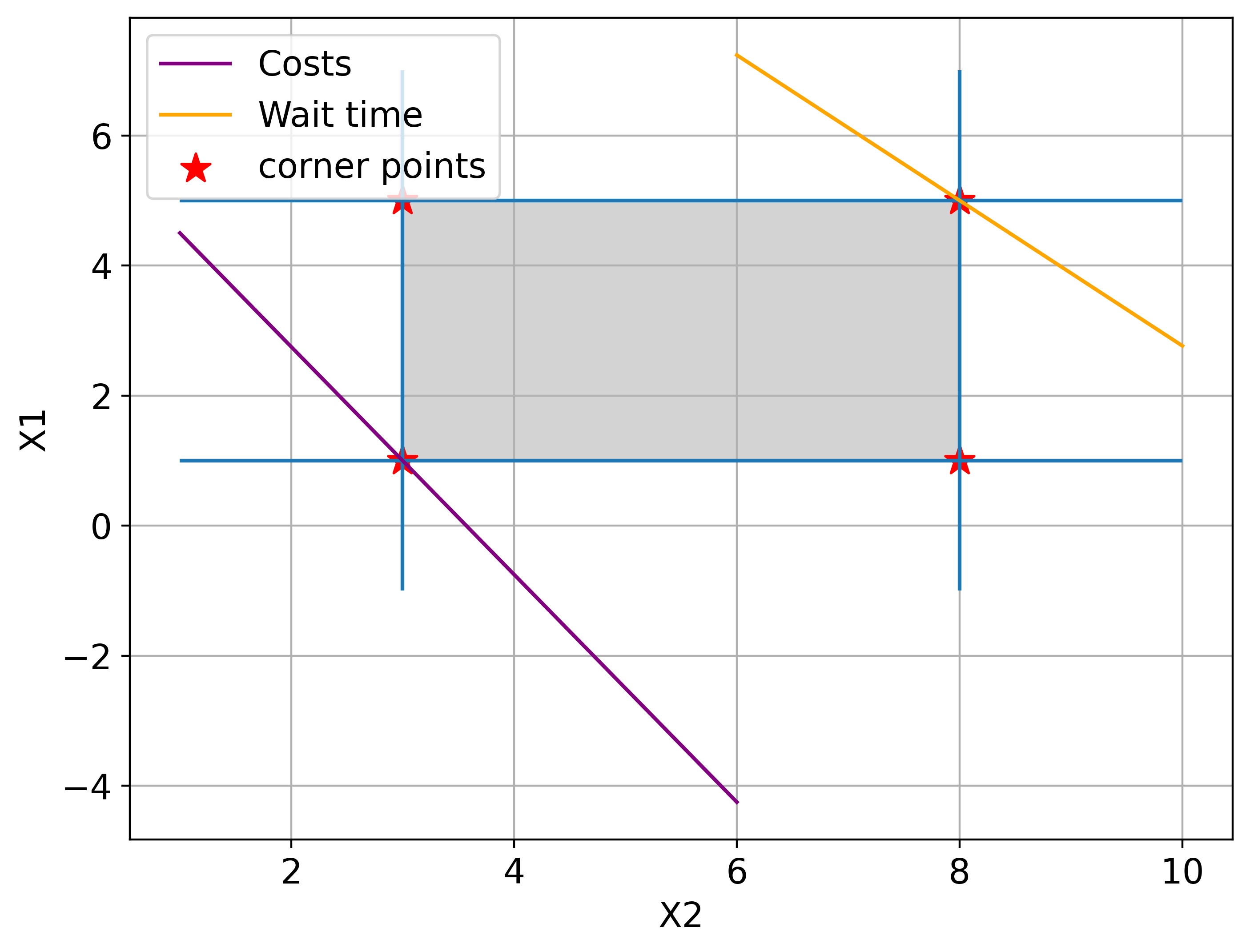
Plot the results#
After optimising using the minimise algorithm the solution space and the objective function are plotted.
# plot graphical solution
fig, ax = plt.subplots(figsize=(8, 6))

# Draw constraint lines
ax.vlines(3, -1, 7)
ax.vlines(8, -1, 7)
ax.hlines(1, 1, 10)
ax.hlines(5, 1, 10)

# Draw the feasible region
feasible_set = Polygon(np.array([[3, 1],
                                 [8, 1],
                                 [8, 5],
                                 [3, 5]]),
                       color="lightgrey")
ax.add_patch(feasible_set)

ax.set_xlabel('X2')
ax.set_ylabel('X1')

# Draw the objective function
x2 = np.linspace(1, 6)
ax.plot(x2, (optimal_result_O1 - c1 * c3 * x2) / (c1 * c2), color="purple", label='Costs')
x2 = np.linspace(6, 10)
ax.plot(x2, (WT0 - c4 * c6 * x2 - optimal_result_O2) / (c4 * c5), color="orange", label='Wait time')

ax.scatter([3,3,8,8], [1,5,1,5], marker='*', color='red', label='corner points', s=150)

ax.legend()
ax.grid()
plt.show();
Corner point evaluation#
Now the corner points of the solution space can be evaluated using the Tetra solver.
# corner point evaluation with Tetra
def preference_P1(variables):
    x1 = variables[:, 0]
    x2 = variables[:, 1]

    costs = objective_costs([x1, x2])
    return 7600 / 51 - 100 * costs / 153

def preference_P2(variables):
    x1 = variables[:, 0]
    x2 = variables[:, 1]

    wait_time = objective_wait_time([x1, x2])
    return 291.747 - 2.67953 * wait_time


alternatives = np.array([
    [1, 3],
    [1, 8],
    [5, 3],
    [5, 8]
])

P1 = preference_P1(alternatives)
P2 = preference_P2(alternatives)

w = [0.5, 0.5] # weights are equal here
p = [P1, P2]

ret = a_fine_aggregator(w, p)

# add results to DataFrame and print it
results = np.zeros((4, 3))
results[:, 0] = alternatives[:, 0]
results[:, 1] = alternatives[:, 1]
results[:, 2] = np.multiply(-1, ret)

df = pd.DataFrame(np.round_(results, 2), columns=['x1', 'x2', 'Aggregated preference'])
print(df)
    x1   x2  Aggregated preference
0  1.0  3.0                  36.68
1  1.0  8.0                   0.00
2  5.0  3.0                 100.00
3  5.0  8.0                  63.32
constants_1 = np.linspace(75, 228)
constants_2 = np.linspace(71.56, 108.88)

pref_1 = 7600 / 51 - 100 * constants_1 / 153
pref_2 = 291.747 - 2.67953 * constants_2

fig = plt.figure()
ax1 = fig.add_subplot(1, 1, 1)
ax1.plot(constants_1, pref_1)
ax1.set_xlim((70, 235))
ax1.set_ylim((0, 100))
ax1.set_title('Costs')
ax1.set_xlabel('Costs [€]')
ax1.set_ylabel('Preference score')
ax1.grid()
plt.show()

fig = plt.figure()
ax2 = fig.add_subplot(1, 1, 1)
ax2.plot(constants_2, pref_2)
ax2.set_xlim((65, 115))
ax2.set_ylim((0, 100))
ax2.set_title('Waiting time')
ax2.set_xlabel('Waiting time [s]')
ax2.set_ylabel('Preference score')
ax2.grid()
plt.show()
A priori optimisation#
The optimisation above initially considers only the single stakeholders and evaluates only the corner points. However, as you will in other examples, this is no guarantee that the optimal solution is found. Here, the optimal point is not on any of the corners. To find the optimal solutions in these cases, a multi-objective optimisation is performed.
The same is showed below for the bridge problem, so you can see how the single-objective optimisations, the multi-objective evaluation, and the multi-objective optimisation relate to each other.
from genetic_algorithm_pfm import GeneticAlgorithm

weights = [0.5, 0.5]

def objective(variables):
    p1 = preference_P1(variables)
    p2 = preference_P2(variables)

    return weights, [p1, p2]

bounds = [[1, 5], [3, 8]]
options = {
    'aggregation': 'a_fine',
    "n_pop": 120,
    "max_stall": 60,
    "n_iter": 1000,
    "n_bits": 8,
    "r_cross": 0.9
}

# run the GA and print its result
ga = GeneticAlgorithm(objective=objective, constraints=[], bounds=bounds, options=options)
score, design_variables, _ = ga.run()

print()
print('Results multi-objective optimisation')
print(f'x1 = {design_variables[0]} and x2 = {design_variables[1]}.')
The type of aggregation is set to a_fine
Generation   Best score   Mean             Max stall    Diversity    Number of non-feasible results
No initial starting point for the optimization with the a-fine-aggregator is given. A random population is generated.
0            -100.0       -34.3212         1            0.017        0
1            -100.0       -79.5951         2            0.188        0
2            -100.0       -79.7827         1            0.342        0
3            -100.0       -91.3552         2            0.221        0
4            -100.0       -91.6844         1            0.429        0
5            -100.0       -92.7016         2            0.412        0
6            -100.0       -89.0771         3            0.392        0
7            -100.0       -91.1093         4            0.421        0
8            -100.0       -95.6549         5            0.446        0
9            -100.0       -94.761          6            0.442        0
10           -100.0       -92.6198         7            0.425        0
11           -100.0       -84.5174         8            0.425        0
12           -100.0       -90.3866         9            0.35         0
13           -100.0       -92.1431         10           0.421        0
14           -100.0       -94.5978         11           0.429        0
15           -100.0       -91.9916         12           0.425        0
16           -100.0       -89.8685         13           0.438        0
17           -100.0       -92.6939         14           0.417        0
18           -100.0       -91.4171         15           0.421        0
19           -100.0       -94.0053         16           0.417        0
20           -100.0       -90.9118         17           0.438        0
21           -100.0       -87.0313         18           0.433        0
22           -100.0       -68.89           19           0.421        0
23           -100.0       -94.6577         20           0.442        0
24           -100.0       -95.8959         21           0.45         0
25           -100.0       -90.9943         22           0.408        0
26           -100.0       -89.2141         23           0.425        0
27           -100.0       -87.5114         24           0.421        0
28           -100.0       -93.4957         25           0.421        0
29           -100.0       -94.2854         26           0.438        0
30           -100.0       -85.2189         27           0.412        0
31           -100.0       -89.1417         28           0.417        0
32           -100.0       -86.0954         29           0.412        0
33           -100.0       -91.0166         30           0.433        0
34           -100.0       -91.7523         31           0.433        0
35           -100.0       -94.0363         32           0.425        0
36           -100.0       -94.1904         33           0.421        0
37           -100.0       -93.8514         34           0.442        0
38           -100.0       -91.0599         35           0.446        0
39           -100.0       -93.6419         36           0.454        0
40           -100.0       -91.6437         37           0.425        0
41           -100.0       -94.4822         38           0.421        0
42           -100.0       -92.8724         39           0.442        0
43           -100.0       -90.2641         40           0.425        0
44           -100.0       -91.014          41           0.438        0
45           -100.0       -93.9772         42           0.442        0
46           -100.0       -90.7165         43           0.412        0
47           -100.0       -87.7539         44           0.417        0
48           -100.0       -76.3443         45           0.438        0
49           -100.0       -91.6208         46           0.425        0
50           -100.0       -83.5065         47           0.4          0
51           -100.0       -86.4593         48           0.392        0
52           -100.0       -88.8302         49           0.396        0
53           -100.0       -88.6736         50           0.421        0
54           -100.0       -87.5807         51           0.446        0
55           -100.0       -91.1472         52           0.392        0
56           -100.0       -87.014          53           0.417        0
57           -100.0       -86.288          54           0.408        0
58           -100.0       -94.611          55           0.429        0
59           -100.0       -93.8426         56           0.429        0
60           -100.0       -91.8967         57           0.4          0
61           -100.0       -90.7563         58           0.425        0
62           -100.0       -93.5012         59           0.433        0
63           -100.0       -94.9854         60           0.442        0
Stopped at gen 63
The number of generations is terribly close to the number of max stall iterations. This suggests a too fast convergence and wrong results.
Please be careful in using these results and assume they are wrong unless proven otherwise!
Execution time was 0.2041 seconds

Results multi-objective optimisation
x1 = 4.984375 and x2 = 3.01953125.
# create figure that shows the results in the design space
plt.rcParams.update({'font.size': 14})
fig, ax = plt.subplots(figsize=(7, 7))
ax.set_xlim((2, 9))
ax.set_ylim((0, 6))
ax.set_xlabel(r'$x_2$ = bridge height')
ax.set_ylabel(r'$x_1$ = bridge span')
ax.set_title('Design space')

# define corner points of design space
x_fill = [3, 8, 8, 3]
y_fill = [1, 1, 5, 5]

ax.fill_between(x_fill, y_fill, color='#539ecd', label='Design space')
ax.scatter(design_variables[1], design_variables[0], label='Optimal solution IMAP', color='tab:purple')

ax.grid()  # show grid
ax.legend()  # show legend
plt.show();  # show figure