5.1. Modules

5.1.1. Python Modules

Previously, you have learned how to:

1) initialize variables in Python;
2) perform simple actions with them (eg.: adding numbers together, displaying variables content, etc);
3) work with functions (have your own code in a function to reuse it many times or use a function, which was written by another person).

However, the scope of the last Notebook was limited by your Python knowledge and available functions in standard/vanilla Python (so-called ’built-in’ Python functions). There are not many Python built-in functions that can be useful for you, such as functions for math, plotting, signal processing, etc. Luckily, there are countless modules/packages written by other people.

5.1.1.1. Python built-in modules

By installing any version of Python, you also automatically install its built-in modules.

One may wonder — why do they provide some functions within built-in modules, but not directly as a built-in function, such as the abs() or print()?

The answers may vary, but, generally, it is to keep your code clean; compact; and, working.

It keeps your code clean and compact as you only load functions that you need. It keeps your code working as it allows you to define your own functions with (almost) any kind of name, and use them easily, without worrying that you might ’break’ something if there is a function with the same name that does something completely different.

5.1.1.2. math

The math module is one of the most popular modules since it contains all implementations of basic math functions (\(sin\), \(cos\), \(exp\), rounding, and other functions — the full list can be found here).

In order to access it, you just have to import it into your code with an import statement. Then using print() to show that math is actually a built-in Python module.

import math
print(math) 

<module 'math' (built-in)>

You can now use its functions like this:

print(f'Square root of 16 is equal to {int(math.sqrt(16))}')

Square root of 16 is equal to 4

You can also use the constants defined within the module, such as math.pi:

print(f'π is equal to {math.pi}')
print('π is equal to {:.2f}'.format(math.pi)) 
print('π is equal to {:.1f}'.format(math.pi))
print('π with two decimals is {:.2f},'
      'with three decimals is {:.3f} and with four decimals is {:.4f}'.\
      format(math.pi, math.pi, math.pi))

π is equal to 3.141592653589793
π is equal to 3.14
π is equal to 3.1
π with two decimals is 3.14,with three decimals is 3.142 and with four decimals is 3.1416

Let’s break it down

• print('π is equal to {:.2f}'.format(math.pi)) print the variable up to some decimal, (two for example).

• print('π is equal to {:.1f}'.format(math.pi)) change the number 2 on the ‘:.2f’ to print with more (or fewer) decimals.

• The last line show how to print is quickly if you have to print a sentence with many variables in it.

More information on printing best practices here.

5.1.1.3. math.pi

As you can see, both constants and functions of a module are accessed by using: the module’s name (in this case math) and a . followed by the name of the constant/function (in this case pi).

We are able to do this since we have loaded all contents of the module by using the import keyword. If we try to use these functions somehow differently — we will get an error:

print('Square root of 16 is equal to')
print(sqrt(16))

Square root of 16 is equal to
4.0

You could, however, directly specify the functionality of the module you want to access. Then, the above cell would work.

This is done by typing: from module_name import necessary_functionality, as shown below:

from math import sqrt

print(f'Square root of 16 is equal to {int(sqrt(16))}.')

Square root of 16 is equal to 4.

from math import pi

print(f'π is equal to {pi}.')

π is equal to 3.141592653589793.

5.1.1.4. Listing all functions

Sometimes, when you use a module for the first time, you may have no clue about the functions inside of it. In order to unveil all the potential a module has to offer, you can either access the documentation on the corresponding web resource or you can use some Python code.

You can listing all contents of a module using dir(). To learn something about, let’s say, hypot thingy you can type the module name - dot -function name, for example math.hypot.

import math
print('contents of math:', dir(math))
print('math hypot is a', math.hypot) 

contents of math: ['__doc__', '__loader__', '__name__', '__package__', '__spec__', 'acos', 'acosh', 'asin', 'asinh', 'atan', 'atan2', 'atanh', 'ceil', 'comb', 'copysign', 'cos', 'cosh', 'degrees', 'dist', 'e', 'erf', 'erfc', 'exp', 'expm1', 'fabs', 'factorial', 'floor', 'fmod', 'frexp', 'fsum', 'gamma', 'gcd', 'hypot', 'inf', 'isclose', 'isfinite', 'isinf', 'isnan', 'isqrt', 'ldexp', 'lgamma', 'log', 'log10', 'log1p', 'log2', 'modf', 'nan', 'perm', 'pi', 'pow', 'prod', 'radians', 'remainder', 'sin', 'sinh', 'sqrt', 'tan', 'tanh', 'tau', 'trunc']
math hypot is a <built-in function hypot>

You can also use ? or ?? to read the documentation about it in Python

math.hypot?

Docstring:
hypot(*coordinates) -> value

Multidimensional Euclidean distance from the origin to a point.

Roughly equivalent to:
    sqrt(sum(x**2 for x in coordinates))

For a two dimensional point (x, y), gives the hypotenuse
using the Pythagorean theorem:  sqrt(x*x + y*y).

For example, the hypotenuse of a 3/4/5 right triangle is:

    >>> hypot(3.0, 4.0)
    5.0
Type:      builtin_function_or_method

5.1.1.5. Python third-party modules

Besides built-in modules, there are also modules developed by other people and companies, which can be also used in your code.

These modules are not installed by default in Python, they are usually installed by using the ’pip’ or ’conda’ package managers and accessed like any other Python module.

This YouTube video explains how to install Python Packages with ’pip’ and ’conda’.

5.1.1.6. numpy

The numpy module is one of the most popular Python modules for numerical applications. Due to its popularity, developers tend to skip using the whole module name and use a smaller version of it (np). A different name to access a module can be done by using the as keyword, as shown below.

import numpy as np
print(np)
x = np.linspace(0, 2 * np.pi, 50)
y = np.cos(x)
print('\n\nx =', x)
print('\n\ny =', y)

<module 'numpy' from 'c:\\ProgramData\\Anaconda3\\lib\\site-packages\\numpy\\__init__.py'>


x = [0.         0.12822827 0.25645654 0.38468481 0.51291309 0.64114136
 0.76936963 0.8975979  1.02582617 1.15405444 1.28228272 1.41051099
 1.53873926 1.66696753 1.7951958  1.92342407 2.05165235 2.17988062
 2.30810889 2.43633716 2.56456543 2.6927937  2.82102197 2.94925025
 3.07747852 3.20570679 3.33393506 3.46216333 3.5903916  3.71861988
 3.84684815 3.97507642 4.10330469 4.23153296 4.35976123 4.48798951
 4.61621778 4.74444605 4.87267432 5.00090259 5.12913086 5.25735913
 5.38558741 5.51381568 5.64204395 5.77027222 5.89850049 6.02672876
 6.15495704 6.28318531]


y = [ 1.          0.99179001  0.96729486  0.92691676  0.8713187   0.80141362
  0.71834935  0.6234898   0.51839257  0.40478334  0.28452759  0.1595999
  0.03205158 -0.09602303 -0.22252093 -0.34536505 -0.46253829 -0.57211666
 -0.67230089 -0.76144596 -0.8380881  -0.90096887 -0.94905575 -0.98155916
 -0.99794539 -0.99794539 -0.98155916 -0.94905575 -0.90096887 -0.8380881
 -0.76144596 -0.67230089 -0.57211666 -0.46253829 -0.34536505 -0.22252093
 -0.09602303  0.03205158  0.1595999   0.28452759  0.40478334  0.51839257
  0.6234898   0.71834935  0.80141362  0.8713187   0.92691676  0.96729486
  0.99179001  1.        ]

Let’s break it down

The code uses the numpy library in Python to perform the following tasks:

1. It imports the numpy library.

2. It prints information about the numpy package.

3. It creates an array x with 50 equally spaced values between \(0\) and \(2\pi\).

4. It calculates the cosine of each element in the array x and stores the results in the array y.

5. It prints the arrays x and y.

In summary, the code imports the numpy library, creates an array x with \(50\) evenly spaced elements between \(0\) and \(2\pi\), calculates the cosine of each element in x, and finally prints the arrays x and y.

You will learn more about this and other packages in separate Notebooks since these packages are frequently used by the scientific programming community.

5.1.1.7. matplotlib

The matplotlib module is used to plot data. It contains a lot of visualization techniques and, for simplicity, it has many submodules within the main module. Thus, in order to access functions, you have to specify the whole path that you want to import.

For example, if the function you need is located within the matplotlib module and pyplot submodule, you need to import matplotlib.pyplot; then, the access command to that function is simply pyplot.your_function().

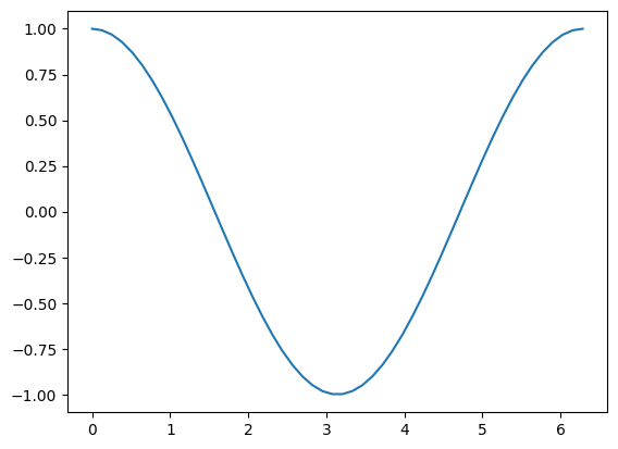
Below we use the data generated in the previous cell to create a simple plot using the pyplot.plot() function:

In order to import a submodule the parent module must also be specified. It is common to import matplotlib.pyplot as plt.

The plt.plot() function takes x-axis values as the first argument and y-axis, or \(f(x)\), values as the second argument

import matplotlib.pyplot as plt
plt.plot(x, y)

[<matplotlib.lines.Line2D at 0x17fff89af70>]

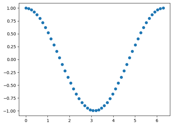
plt.scatter() works in a similar way, but it does not connect the dots.

plt.scatter(x, y)

<matplotlib.collections.PathCollection at 0x17fff8f4f40>

5.1.1.8. Loading Python files as modules

Finally, you can also load your own (or somebody else’s) Python files as modules. This is quite helpful, as it allows you to keep your code projects well-structured without the need to copy and paste everything.

In order to import another *.py file as a module, you only need to have that file and your Notebook file in the same directory and use the import keyword. More info on this here.

5.1.2. Additional study material

• Official Python Documentation - https://docs.python.org/3/tutorial/modules.html

• https://realpython.com/python-modules-packages/

• Think Python (2nd ed.) - Sections 3 and 14

5.1.2.1. After this Notebook you should be able to:

• understand the difference between built-in and third-party modules

• use functions from the math module

• find available functions from any module

• generate an array for the x-axis

• calculate the cos or sin of the x-axis

• plot such functions

• understand how to load Python files as modules