SymPy for solving Euler-Bernoulli#
SymPy can be used to solve the Euler-Bernoulli’s beam theory. It will take over the cumbersome handcalculations. However the engineering part; the thinking, the modelling and the correct input of the specifications still remains a human matter.
A simple beam is taken as an example. The beam is loaded with a uniform load \(q\) on a part of the beam and a force \(F\). The beam is a prismatic beam with a bending stiffness \(EI\).

We can solve this beam by using the Euler-Bernoulli’s differential equation. This page will focus solely on the implementations of those calculations in SymPy. Click –> Live Code to activate live coding on this page!
First, the SymPy library is imported:
import sympy as sym
sym.init_printing()
import sympy as sym
Now, we’ll define our symbols. These includes all symbols (non-numerical values), so also including intergration constants. We do so with the sym.symbols function:
x, q, F, EI = sym.symbols('x, q, F, EI')
C1, C2, C3, C4, C5, C6, C7, C8, C9, C10, C11, C12 = sym.symbols('C1 C2 C3 C4 C5 C6 C7 C8 C9 C10 C11 C12')
The functions \(q\left(x\right)\) for each of the segments can now be defined:
q_AC = q
q_CD = 0
q_DB = 0
We can integrate using the sym.integrate() function:
V_AC = sym.integrate(-q_AC,x)+C1
M_AC = sym.integrate(V_AC,x)+C2
kappa_AC = M_AC / EI
phi_AC = sym.integrate(kappa_AC,x)+C3
w_AC = sym.integrate(-phi_AC,x)+C4

V_CD = sym.integrate(-q_CD,x)+C5
M_CD = sym.integrate(V_CD,x)+C6
kappa_CD = M_CD / EI
phi_CD = sym.integrate(kappa_CD,x)+C7
w_CD = sym.integrate(-phi_CD,x)+C8

V_DB = sym.integrate(-q_DB,x)+C9
M_DB = sym.integrate(V_DB,x)+C10
kappa_DB = M_DB / EI
phi_DB = sym.integrate(kappa_DB,x)+C11
w_DB = sym.integrate(-phi_DB,x)+C12
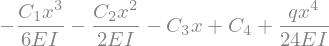
You can display the equations with the display function:
display(w_AC)
The boundary conditions can now be specified using the sym.Eq() function which takes as an input the left- and righthandside of an equation. Furthermore the .subs() function fill in a value in your expression:
Eq1 = sym.Eq(w_AC.subs(x, 0), 0)
Eq2 = sym.Eq(M_AC.subs(x, 0), 0)
Eq3 = sym.Eq(w_AC.subs(x, 4), w_CD.subs(x, 4))
Eq4 = sym.Eq(phi_AC.subs(x, 4), phi_CD.subs(x, 4))
Eq5 = sym.Eq(M_AC.subs(x, 4), M_CD.subs(x, 4))
Eq6 = sym.Eq(V_AC.subs(x, 4), V_CD.subs(x, 4))
Eq7 = sym.Eq(w_CD.subs(x, 9), w_DB.subs(x, 9))
Eq8 = sym.Eq(phi_CD.subs(x, 9), phi_DB.subs(x, 9))
Eq9 = sym.Eq(V_CD.subs(x, 9), V_DB.subs(x, 9)+F)
Eq10 = sym.Eq(M_CD.subs(x, 9), M_DB.subs(x, 9))
Eq11 = sym.Eq(w_DB.subs(x, 15), 0)
Eq12 = sym.Eq(M_DB.subs(x, 15), 0)

display(Eq7)

Now we use the function sym.solve to solve our system of equations for our integration constants:
sol = sym.solve((Eq1,Eq2,Eq3,Eq4,Eq5,Eq6,Eq7,Eq8,Eq9,Eq10,Eq11,Eq12), (C1,C2,C3,C4,C5,C6,C7,C8,C9,C10,C11,C12))
display(sol)

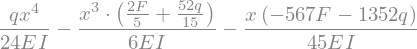
We can use .subs() again to substitute this solution in our original function:
display(w_AC.subs(sol))
Instead of symbolic values, you could have worked with numerical values too from the beginning. Nevertheless, we can substitute some random values with out final expression too, including a value for x. Use .evalf() to show the decimal form of your answer:
display(w_CD.subs(sol).subs(EI,50000).subs(q,10).subs(F,35).subs(x,6))
display(w_CD.subs(sol).subs(EI,50000).subs(q,10).subs(F,35).subs(x,6).evalf())


You can plot the results too. The details of how to make plot is not covered here (if you’re curious, the book Python for Engineers might help you). On this page, you can use the function plot(), with a list of functions to plot and a list of domains over which to plot those functions:
import numpy as np
import matplotlib.pyplot as plt

%config InlineBackend.figure_formats = ['svg']

def plot(w_list, x_range_list,ylabel):
    plt.figure()
    for i, w in enumerate(w_list):
        # check if x is the only symbol in the expression
        if len(w.free_symbols) > 1:
            raise ValueError('The expression must be a function of x only.')

        w_numpy = sym.lambdify(x, w)
        x_vals = np.linspace(x_range_list[i][0], x_range_list[i][1], 100)

        # if the expression is a constant, we need to make sure that it is broadcasted correctly
        if isinstance(w_numpy(x_vals),float) or isinstance(w_numpy(x_vals),int):
            w_numpy = np.vectorize(w_numpy)
            plt.plot([x_range_list[i][0], x_range_list[i][1]],[w_numpy(x_vals),w_numpy(x_vals)])
        else:
            plt.plot(x_vals,w_numpy(x_vals))

        plt.plot(x_vals,w_numpy(x_vals))
        plt.xlabel('$x$')
        plt.ylabel(ylabel)
    ax = plt.gca()
    ax.spines['right'].set_color('none')
    ax.spines['top'].set_color('none')
    ax.spines['bottom'].set_position('zero')
    ax.spines['left'].set_position('zero')
    ax.invert_yaxis()
plot([w_AC.subs(sol).subs(EI,50000).subs(q,10).subs(F,35), w_CD.subs(sol).subs(EI,50000).subs(q,10).subs(F,35), w_DB.subs(sol).subs(EI,50000).subs(q,10).subs(F,35)], [[0, 4],[4, 9],[9, 15]],'w(x)')

plot([M_AC.subs(sol).subs(q,10).subs(F,35), M_CD.subs(sol).subs(q,10).subs(F,35), M_DB.subs(sol).subs(q,10).subs(F,35)], [[0, 4],[4, 9],[9, 15]],'M(x)')

Exercises#
Exercises are available in chapter 8.6 of the book Engineering Mechanics Volume 2 (Hartsuijker and Welleman, 2006): 8.7 - 8.11, 8,26 - 8.31, 8.34 - 8.37. Try to solve these exercises using Python and Sympy, or another numerical tool you master.
If you don’t have Python and SymPy installed, click –> Live Code to activate live coding and use the cells below:
import sympy as sym
sym.init_printing()
x = sym.symbols('x')
C1, C2, C3, C4 = sym.symbols('C1 C2 C3 C4')
q =
V = sym.integrate(-q,x)+C1
M = sym.integrate(V,x)+C2
kappa = M / EI
phi = sym.integrate(kappa,x)+C3
w = sym.integrate(-phi,x)+C4
Eq1 = sym.Eq(
sol = sym.solve((Eq1,Eq2,Eq3,Eq4,Eq5,Eq6,Eq7,Eq8,Eq9,Eq10,Eq11,Eq12), (C1,C2,C3,C4,C5,C6,C7,C8,C9,C10,C11,C12))
display(sol)
M.subs(sol)
import numpy as np
import matplotlib.pyplot as plt

%config InlineBackend.figure_formats = ['svg']

def plot(w_list, x_range_list,ylabel):
    plt.figure()
    for i, w in enumerate(w_list):
        # check if x is the only symbol in the expression
        if len(w.free_symbols) > 1:
            raise ValueError('The expression must be a function of x only.')

        w_numpy = sym.lambdify(x, w)
        x_vals = np.linspace(x_range_list[i][0], x_range_list[i][1], 100)

        # if the expression is a constant, we need to make sure that it is broadcasted correctly
        if isinstance(w_numpy(x_vals),float) or isinstance(w_numpy(x_vals),int):
            w_numpy = np.vectorize(w_numpy)
            plt.plot([x_range_list[i][0], x_range_list[i][1]],[w_numpy(x_vals),w_numpy(x_vals)])
        else:
            plt.plot(x_vals,w_numpy(x_vals))

        plt.plot(x_vals,w_numpy(x_vals))
        plt.xlabel('$x$')
        plt.ylabel(ylabel)
    ax = plt.gca()
    ax.spines['right'].set_color('none')
    ax.spines['top'].set_color('none')
    ax.spines['bottom'].set_position('zero')
    ax.spines['left'].set_position('zero')
    ax.invert_yaxis()
plot(