14.1. Reliability index \(\beta\)

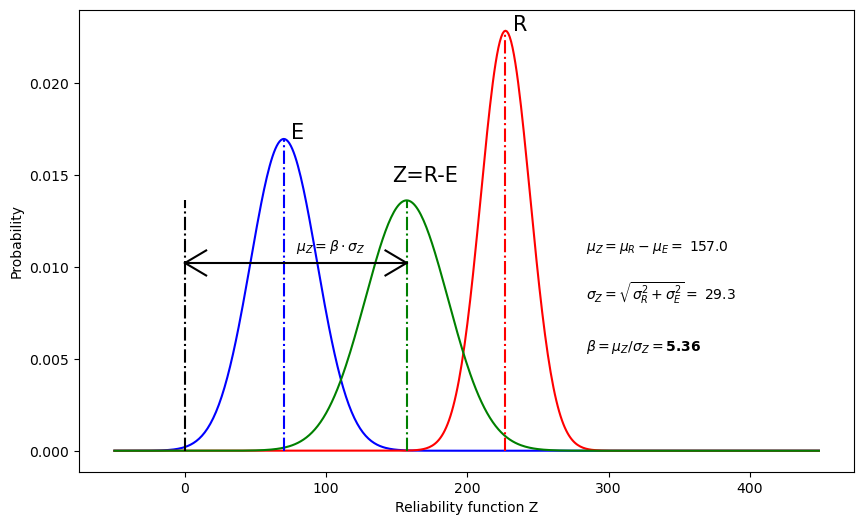
In section Structural safety we have seen the definition of the reliability factor \(\beta\), using a symbolic approach. Now, we will show some examples with values as well as python-implementation to produce graphs and show dynamic graphs. For the first example, we have chosen the average strength R to be \(\mu_{R}=227\), and have assumed this strength has a normal distribution with standard deviation \(\sigma_{R}=17.46\). The unit is not relevant for the example; it could be any unit of force or stress, as long as Effects E and Resistance R are expressed in the same unit. Now let’s also assume this fictitious structure is loaded by some Effect E that results in force in stress in our structure. Of E we assume that its’ average is \(\mu_{E}=70\) and SD is \(\sigma_{E}=23.5\). For the structure being sufficiently safe, E should be smaller than or equal to R with sufficiently high probability.

Fig. 14.1 E, R, and Z function with numerical example

We see that \(\beta=5.36\), which, according to Table 2.1, represents a probability of failure \(P_f\) between \(10^{-7}\) and \(10^{-8}\). Now try for yourself:

Exercise

If \(\mu_E = 100\), \(\sigma_E = 20\), \(\mu_R = 240\) and \(\sigma_R = 20\), what are \(\mu_Z\), \(\sigma_Z\) and \(\beta\)?

You might want to download some code cells or the full .ipynb page and put code in there to perform the calculations, and plot the graphs.

Solution

\(\mu_Z = \mu_R - \mu_E = 140\)
\(\sigma_Z = \sqrt{\sigma_R^2 + \sigma_E^2} = 22.4\)
\(\beta = \frac{\mu_Z}{\sigma_Z} = 6.3\)

Code to generate reliability function Z

Using the Python code below, you play with the numerical values yourself:

import numpy as np
import math
import matplotlib.pyplot as plt
from scipy.stats import norm
import statistics

def plot_Z(meanE, sdE, meanR, sdR):
    
    # define lower and upper values of Effect E and Resistance R
    Elower = 0.5*meanE
    Eupper = 1.5*meanE
    E = np.arange(Elower, Eupper, 1)
    Rlower = 0.85*meanR
    Rupper = 1.15*meanR
    R = np.arange(Rlower, Rupper, 1)

    # Plot x-axis range with 1 steps
    x_axis = np.arange(-50, 450, 1)

    # figure size in inches
    plt.figure(figsize=(10, 6))

    # Calculating statistics
    probE = (1 / (sdE * math.sqrt(2 * math.pi))) * math.exp(-((0) ** 2) / (2 * sdE ** 2))
    probErep = (1 / (sdE * math.sqrt(2 * math.pi))) * math.exp((-(1.64 * sdE) ** 2) / (2 * sdE ** 2))
    
    probR = (1 / (sdR * math.sqrt(2 * math.pi))) * math.exp(-((0) ** 2) / (2 * sdR ** 2))
    probRrep = (1 / (sdR * math.sqrt(2 * math.pi))) * math.exp((-(1.64 * sdR) ** 2) / (2 * sdR ** 2))
        
    # calculation reliability function
    meanZ = meanR-meanE
    sdZ=math.sqrt(sdE**2+sdR**2)
    probZ=(1/(sdZ*math.sqrt(2*math.pi)))*math.exp(-((0)**2)/(2*sdZ**2))
    beta=meanZ/sdZ

    # plot normal distribution curves for E (blue) and R (red) and Z (green)
    plt.plot(x_axis, norm.pdf(x_axis, meanE, sdE), 'b')
    plt.plot(x_axis, norm.pdf(x_axis, meanR, sdR), 'r')
    plt.plot(x_axis, norm.pdf(x_axis, meanZ, sdZ), 'g')

    # plot averages with dash-dotted red/blue lines
    plt.plot([meanR, meanR], [0, probR], 'r-.')
    plt.plot([meanE, meanE], [0, probE], 'b-.')
    plt.plot([meanZ,meanZ],[0,probZ], 'g-.')
    
    plt.text(meanE + 5, probE, 'E', fontsize=15)
    plt.text(meanR + 5, probR, 'R', fontsize=15)
    plt.text(meanZ-10, probZ+0.001, 'Z=R-E', fontsize=15)

    # arrows for beta
    plt.plot([0,0],[0,probZ], 'k-.')
    plt.plot([0,meanZ],[0.75*probZ,0.75*probZ], 'k-')
    plt.plot([0,15],[0.75*probZ,0.80*probZ], 'k-')
    plt.plot([0,15],[0.75*probZ,0.70*probZ], 'k-')
    plt.plot([meanZ,meanZ-15],[0.75*probZ,0.80*probZ], 'k-')
    plt.plot([meanZ,meanZ-15],[0.75*probZ,0.70*probZ], 'k-')
    plt.text(meanZ/2, 0.8*probZ, "$\\mu_Z = \\beta \\cdot \\sigma_Z $", fontsize=10)
    plt.text(meanR*1.25, 0.8*probZ, "$\\mu_Z = \\mu_R - \mu_E =$ "+'{0:.1f}'.format(meanZ), fontsize=10)
    plt.text(meanR*1.25, 0.60*probZ, "$\\sigma_Z = \sqrt{\sigma_R^2 + \sigma_E^2} =$ "+'{0:.1f}'.format(sdZ), fontsize=10)
    plt.text(meanR*1.25, 0.40*probZ, "$\\beta = \\mu_Z / \\sigma_Z = $"+'{0:.2f}'.format(beta), fontsize=10, fontweight='bold')


    plt.xlabel("Reliability function Z")
    plt.ylabel("Probability")

    # plt.savefig("Z_curve.pdf", format="pdf", bbox_inches="tight")
    plt.show()

Initializing example with data

Using the functions and numerical values defined above, now plots can be generated:

meanE = 70
sdE = 23.52
meanR = 227
sdR = 17.46

plot_Z(meanE, sdE, meanR, sdR)

Dynamic graphs of \(\beta\) and u.c.

Using the dynamic graphs below, you can see what the influence is of modifying the values for \(\mu_R\) or \(\sigma_R\) on the magnitude of \(\beta\) and the unity check u.c.:

The dynamic graph illustrates the following: if the average of the blue R-function shifts to a lower value, the reliability index \(\beta\) becomes smaller, and the unity check becomes larger. If the average of the blue R-function shifts to a higher value, the reliability index \(\beta\) becomes larger, and the unity check becomes smaller.

The dynamic graph above illustrates the following: if the performance (capacity, resistance) of a material becomes more uncertain, e.g. due to a wider spread of test results of material properties or due to a wider spread of cross-sectional dimensions, \(\sigma_R\) becomes larger. Even without change of the average value \(\mu_R\), the safety of the structure will become lower (value of \(\beta\) drops and u.c. increases). Vice versa, with smaller spread of R, safety will increase.