The information on this page gives a summary of the Loads and Reliability reader, which is part of the safety content of the module CIEM5000 - Structural Engineering Track Base, written by Roel Schipper. In the end an implementation in Python on reliability plots based on his GitHub repository will be given.
A structure should be sufficiently safe. This means that the probability of failure should be sufficiently low, but unfortunately enough it can never be 0 %. It is possible to determine the risk of failure of a structure (or more positively formulated: the structural reliability ) by carrying out a probabilistic calculation. There are 3 methods of calculations to deal with uncertainty, with increasing level of complexity (International Organization for Standardization 11 2015). Those are:
Semi-probabilistic approach: Safety format prescribing the design equations and the analysis procedures to be used default method in the Eurocodes, i.e. to be used for usual design situations.
Reliability-based design and assessment: Reliability requirements to fulfil unusual design situations in regard to uncertainties, code calibration.
Risk-informed decision making: Decisions are taken with due consideration of the total risks (e.g. loss of lives, injuries). Exceptional design situations in regard to uncertainties and consequences. Derivation of reliability requirements.
The annual probability of failure \(P_{f;a}\) and the annual reliability index \(\beta_{a}\) are used in the Eurocode as the two standard metrics to express structural reliability in the semi-probabilistic approach. The index \(a\) (annum) is often left out, since variable loads are represented by the probability distributions of their yearly extreme values. The table below provides the values for both metrics:
Table 2.1 Relation between failure probability \(P_{f}\) and reliability index \(\beta\) (prNEN-EN-1990 2021, table C.2).#
\(P_f\)
\(\beta\)
\(10^{-1}\)
1.28
\(10^{-2}\)
2.33
\(10^{-3}\)
3.09
\(10^{-4}\)
3.72
\(10^{-5}\)
4.26
\(10^{-6}\)
4.75
\(10^{-7}\)
5.2
\(10^{-8}\)
5.61
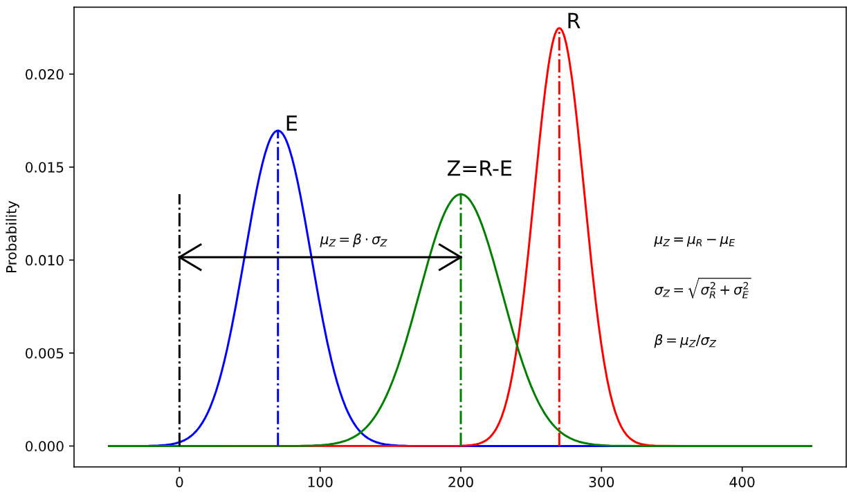
The reliability index \(\beta\) can be calculated from the probaility density functions (PDF) of loads (Effects) and strength (Resistance), shown in the figure below:
Fig. 2.1 Effects vs. Resistance and reliability function Z#
We see in red a PDF curve R which represents the probability that the Resistance (= strength) of a fictitious structure has a given value. We also see a blue PDF curve E (= Effects = loads) of the load on our structure. The green curve Z represents the difference of the E and R curves:
\[
Z=R-E
\]
with
\[
\mu_Z=\mu_R-\mu_E
\]
and
\[
\sigma_Z=\sqrt{\sigma_R^2-\sigma_E^2}
\]
The reliability index \(\beta\) of the structure can now be calculated from the PDFs of E and R:
\[
\beta=\frac{\mu_Z}{\sigma_Z}
\]
Finally, the probability of failure can be derived from the calculated \(\beta\) using Table 2.1 above. Numerical examples and the effects of changes in \(\mu\) or \(\sigma\) of E and R can be found in section Section 14.1.
To prevent that the design of every single structure results in a fully probabilistic undertaking, however, for most structures a simplified approach is allowed. Eurocode 0 (prNEN-EN-1990 2021) describes such a simplified, semi-probabilistic method, in which the stochastic distributions of material strength and load values are expressed by characteristic values, taking into account their spread, and by partial safety factors, that ensure appropriate safety margin between loads and capacity. This safety distance becomes larger for important structures where the consequences of failure are big, and vice versa.
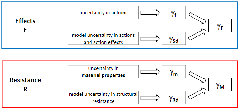
The Eurocode defines partial factors for the Effects side (actions) in the prNEN-EN-1990 (2021), while the partial factors on the Resistance side (materials) are defined in the various material codes for steel, concrete, timber, and so forth. This Load/Resistance Factor (LRF) or split factor format approach is used to allocate the different uncertainty of loads (effects) and uncertainty of resistance (strength) where they belong, that is in separate calculations of design values of loads and resistance, respectively.
Fig. 2.2 Partial factors on Effects-side and Resistance side combine various types of uncertainties#
In depth review of partial factors from Eurocode
How are the values of \(\gamma_{F}\) and \(\gamma_{M}\) related to the stochastic spread? From Schneider and Vrouwenvelder [1] the following equations can be derived:
\(\gamma_i\): partial safety factor for i (i can be E or R)
\(\mu_i\): mean value of i
\(\alpha_i\): weighing factor depending on how dominant the factor is for the reliability of the structure, often \(\alpha_R = 0.8\) for the most dominant resistance variable, \(\alpha_R = 0.32\) for other (non-dominant) resistance variables, \(\alpha_E = -0.7\) for the most dominant load variable or \(\alpha_E = -0.28\) for non-dominant load variables.
\(\beta_0\): required (targeted) reliability index
The general objective of calculations overseeing safety is that the resistance of the structure should be greater than the effect of the load. A useful way to express this is the unity check (u.c.) according to equation (2.1):
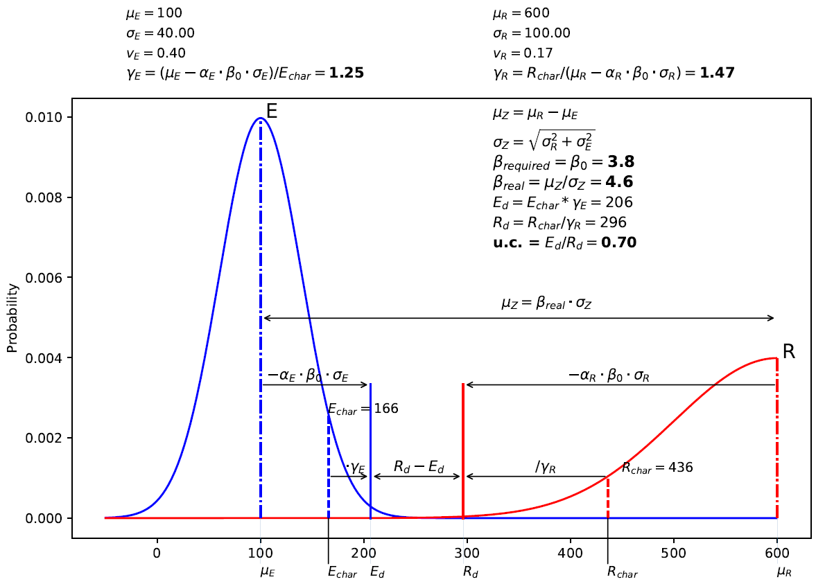
This unity check is obtained in four steps. Fig. 2.3 below gives good visual insight in the steps.
Both effect \(E\) and resistance \(R\) are expressed in their characteristic values. \(E_{char}\) means that the value \(E\) is set a a load level of which the probability of exceedance (overshoot) is 5%. In a similar way \(R_{char}\) is the value with a probability of 5% to undershoot. This is a standard statistic operation that is done by adding or subtracting \(1.64\cdot\sigma\) in case of a normal distribution:
\[
E_{char} = \mu_E + 1.64 \cdot \sigma_E
\]
\[
R_{char} = \mu_R - 1.64 \cdot \sigma_R
\]
See the MUDE online textbook for more explanation and a nice animation of the Gaussian distribution. For loads or materials other distributions may apply, such as Weibull or lognormal distributions.
On the Effect side, \(γ_E\) , the partial load factor, is multiplied with the characteristic value of the load or Effect, resulting in a dimensioning value of \(E\)(2.2), represented by the blue drawn line, and for this example the value \(E_d\) = 163 (again, unit does not matter here, as long as both \(R\) and \(E\) are expressed in the same unit).
On the Resistance side, the characteristic value of the strength or Resistance is divided by \(γ_R\), the partial material factor, resulting in a dimensioning value of \(R\)(2.3), represented by the red drawn line, and for this example the value \(R_d = 201\) (same unit as \(E\)).
Finally, \(E_d\) and \(R_d\) are compared, in either of the two following ways: direct comparison \(E_d ≤ R_d\) or unity check equation (2.1), the latter with the advantage that it gives numerical information on the “safety distance” between \(E_d\) and \(R_d\).
Fig. 2.3 Graphical representation of symbols and quantities in the EC semi-probabilistic approach#
Example of a normal distribution of Effects (\(E\)) and Resistance (\(R\)) and the place of characteristic values \(E_{char}\) and \(R_{char}\) and design values \(E_d\) and \(R_d\). The characteristic values are obtained by finding from the normal distribution the values with a 5% probability of exceedance (\(μ_E\) + 1.64 · \(σ_E\) for \(E\) and \(μ_R\) − 1.64 · \(σ_R\) for \(R\)). The design values are found by multiplying /dividing the characteristic values with the partial safety factors \(γ_E\) and \(γ_R\). The distance on the horizontal axis between \(E_d\) and \(R_d\) represents a measure of the unity-check (u.c.). In this example, \(E_d\) = 0.70 · \(R_d\). The structure is more than safe.
If you want to see some numerical examples using the concepts of safety and Python codes to produce the graphs, you can find these under unity_check_example and Section 14.1.