14.1. Effect vs Resistance

import numpy as np
import math
import matplotlib.pyplot as plt
from scipy.stats import norm
import statistics

Effect vs Resistance plotting function

def plot_effect_vs_resistance(meanE, sdE, gamma_E, meanR, sdR, gamma_R):
    # define lower and upper values of Effect E and Resistance R
    Elower = 0.5*meanE
    Eupper = 1.5*meanE
    E = np.arange(Elower, Eupper, 1)
    Rlower = 0.85*meanR
    Rupper = 1.15*meanR
    R = np.arange(Rlower, Rupper, 1)

    # Plot x-axis range with 1 steps
    x_axis = np.arange(-50, 450, 1)

    # figure size in inches
    plt.figure(figsize=(10, 6))

    # Calculating statistics
    probE = (1 / (sdE * math.sqrt(2 * math.pi))) * math.exp(-((0) ** 2) / (2 * sdE ** 2))
    probErep = (1 / (sdE * math.sqrt(2 * math.pi))) * math.exp((-(1.64 * sdE) ** 2) / (2 * sdE ** 2))
    plt.text(Eupper, probE - 0.0015, "$\mu_E=$" + '{0:.0f}'.format(meanE), fontsize=10)
    plt.text(Eupper, probE - 0.003, "$\sigma_E=$" + '{0:.2f}'.format(sdE), fontsize=10)
    plt.text(Eupper, probE - 0.0045, "$\gamma_E=$" + '{0:.2f}'.format(gamma_E), fontsize=10)
    Ed = (meanE + 1.64 * sdE) * gamma_E

    probR = (1 / (sdR * math.sqrt(2 * math.pi))) * math.exp(-((0) ** 2) / (2 * sdR ** 2))
    probRrep = (1 / (sdR * math.sqrt(2 * math.pi))) * math.exp((-(1.64 * sdR) ** 2) / (2 * sdR ** 2))
    plt.text(Rupper, probR - 0.0015, "$\mu_R=$" + '{0:.0f}'.format(meanR), fontsize=10)
    plt.text(Rupper, probR - 0.003, "$\sigma_R=$" + '{0:.2f}'.format(sdR), fontsize=10)
    plt.text(Rupper, probR - 0.0045, "$\gamma_R=$" + '{0:.2f}'.format(gamma_R), fontsize=10)
    Rd = (meanR - 1.64 * sdR) / gamma_R

    # plot Ed values
    plt.text(Rupper * 1.1, 0.5 * probR - 0.0075, "$E_d = E_{char}*\gamma_E=$" + '{0:.0f}'.format(Ed), fontsize=10)
    plt.text(Rupper * 1.1, 0.5 * probR - 0.0090, "$R_d = R_{char}/\gamma_R=$" + '{0:.0f}'.format(Rd), fontsize=10)
    plt.text(Rupper * 1.1, 0.5 * probR - 0.0105, "u.c. = $E_d / R_d = $" + '{0:.2f}'.format(Ed / Rd), fontsize=10)

    # plot normal distribution curves for E (blue) and R (red)
    plt.plot(x_axis, norm.pdf(x_axis, meanE, sdE), 'b')
    plt.plot(x_axis, norm.pdf(x_axis, meanR, sdR), 'r')

    plt.text(meanE + 5, probE, 'E', fontsize=15)
    plt.text(meanE + 1.64 * sdE, probErep, "$E_{char}=$" + '{0:.0f}'.format(meanE + 1.64 * sdE), fontsize=10)
    plt.text(meanE + 2.8 * sdE * gamma_E, probErep * 0.7, '$E_d$', fontsize=10)


    # plot 5%-characteristic value with dashed red/blue lines
    plt.plot([meanR - 1.64 * sdR, meanR - 1.64 * sdR], [0, probRrep], 'r--')
    plt.plot([meanE + 1.64 * sdE, meanE + 1.64 * sdE], [0, probErep], 'b--')

    # plot dimensioning value with drawn red/blue lines
    plt.plot([(meanR - 1.64 * sdR) / gamma_R, (meanR - 1.64 * sdR) / gamma_R], [0, 0.7 * probErep], 'r-')
    plt.plot([(meanE + 1.64 * sdE) * gamma_E, (meanE + 1.64 * sdE) * gamma_E], [0, 0.7 * probErep], 'b-')

    plt.text(meanR + 5, probR, 'R', fontsize=15)
    plt.text(meanR - 3.7 * sdR, probRrep, "$R_{char}=$" + '{0:.0f}'.format(meanR - 1.64 * sdR), fontsize=10)
    plt.text(meanR - 4.5 * sdR / gamma_R, probErep * 0.7, '$R_{d}$', fontsize=10)

    plt.xlabel("Effect (E, left) vs. Resistance (R, right) [unit could be e.g. load in kN or stress in MPa]")
    plt.ylabel("Probability")

    # plt.savefig("E_R_curves_highgamma_uc0.81_beta6_8.pdf", format="pdf", bbox_inches="tight")
    plt.show()

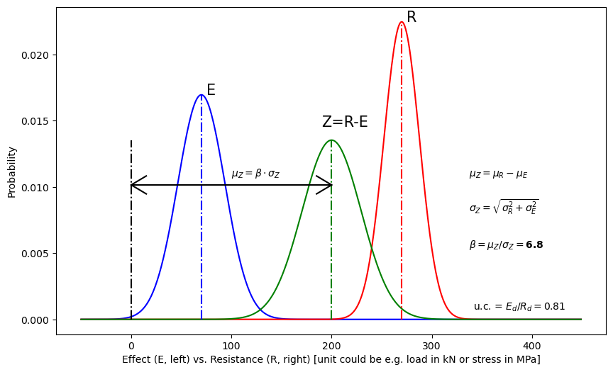
Reliability Z function

def plot_Z(meanE, sdE, gamma_E, meanR, sdR, gamma_R):
    # define lower and upper values of Effect E and Resistance R
    Elower = 0.5*meanE
    Eupper = 1.5*meanE
    E = np.arange(Elower, Eupper, 1)
    Rlower = 0.85*meanR
    Rupper = 1.15*meanR
    R = np.arange(Rlower, Rupper, 1)

    # Plot x-axis range with 1 steps
    x_axis = np.arange(-50, 450, 1)

    # figure size in inches
    plt.figure(figsize=(10, 6))

    # Calculating statistics
    probE = (1 / (sdE * math.sqrt(2 * math.pi))) * math.exp(-((0) ** 2) / (2 * sdE ** 2))
    probErep = (1 / (sdE * math.sqrt(2 * math.pi))) * math.exp((-(1.64 * sdE) ** 2) / (2 * sdE ** 2))
    Ed = (meanE + 1.64 * sdE) * gamma_E

    probR = (1 / (sdR * math.sqrt(2 * math.pi))) * math.exp(-((0) ** 2) / (2 * sdR ** 2))
    probRrep = (1 / (sdR * math.sqrt(2 * math.pi))) * math.exp((-(1.64 * sdR) ** 2) / (2 * sdR ** 2))
    Rd = (meanR - 1.64 * sdR) / gamma_R
    
    # calculation reliability function
    meanZ = meanR-meanE
    sdZ=math.sqrt(sdE**2+sdR**2)
    probZ=(1/(sdZ*math.sqrt(2*math.pi)))*math.exp(-((0)**2)/(2*sdZ**2))
    beta=meanZ/sdZ

    # plot Ed values
    plt.text(Rupper * 1.1, 0.5 * probR - 0.0105, "u.c. = $E_d / R_d = $" + '{0:.2f}'.format(Ed / Rd), fontsize=10)

    # plot normal distribution curves for E (blue) and R (red)
    plt.plot(x_axis, norm.pdf(x_axis, meanE, sdE), 'b')
    plt.plot(x_axis, norm.pdf(x_axis, meanR, sdR), 'r')
    plt.plot(x_axis, norm.pdf(x_axis, meanZ, sdZ), 'g')


    # plot averages with dash-dotted red/blue lines
    plt.plot([meanR, meanR], [0, probR], 'r-.')
    plt.plot([meanE, meanE], [0, probE], 'b-.')
    plt.plot([meanZ,meanZ],[0,probZ], 'g-.')
    
    plt.text(meanE + 5, probE, 'E', fontsize=15)
    plt.text(meanR + 5, probR, 'R', fontsize=15)
    plt.text(meanZ-10, probZ+0.001, 'Z=R-E', fontsize=15)

    # arrows for beta
    plt.plot([0,0],[0,probZ], 'k-.')
    plt.plot([0,meanZ],[0.75*probZ,0.75*probZ], 'k-')
    plt.plot([0,15],[0.75*probZ,0.80*probZ], 'k-')
    plt.plot([0,15],[0.75*probZ,0.70*probZ], 'k-')
    plt.plot([meanZ,meanZ-15],[0.75*probZ,0.80*probZ], 'k-')
    plt.plot([meanZ,meanZ-15],[0.75*probZ,0.70*probZ], 'k-')
    plt.text(meanZ/2, 0.8*probZ, "$\\mu_Z = \\beta \\cdot \\sigma_Z $", fontsize=10)
    plt.text(meanR*1.25, 0.8*probZ, "$\\mu_Z = \\mu_R - \mu_E $", fontsize=10)
    plt.text(meanR*1.25, 0.60*probZ, "$\\sigma_Z = \sqrt{\sigma_R^2 + \sigma_E^2} $", fontsize=10)
    plt.text(meanR*1.25, 0.40*probZ, "$\\beta = \\mu_Z / \\sigma_Z = $"+'{0:.1f}'.format(beta), fontsize=10, fontweight='bold')


    plt.xlabel("Effect (E, left) vs. Resistance (R, right) [unit could be e.g. load in kN or stress in MPa]")
    plt.ylabel("Probability")

    # plt.savefig("E_R_curves_highgamma_uc0.81_beta6.8.pdf", format="pdf", bbox_inches="tight")
    plt.show()

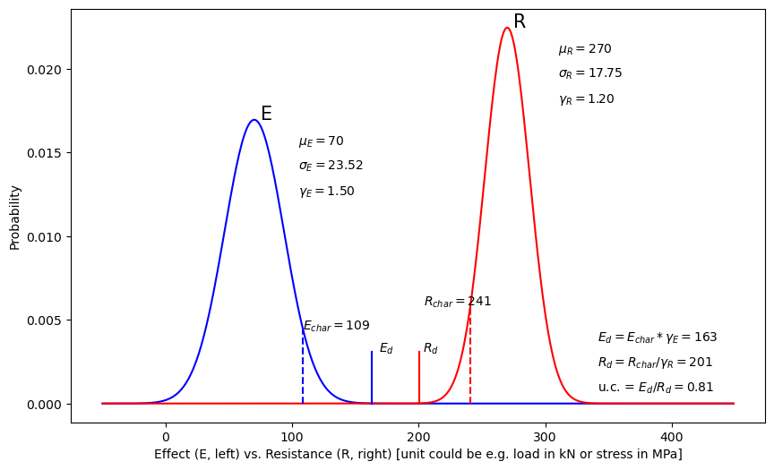
Initializing examples with data

Using the functions defined above, plots can be generated. To do so, we need numerical input values. The numerical values for the example plot above are defined below and the functions executed.

meanE = 70
sdE = 23.52
gamma_E = 1.5

meanR = 270
sdR = 17.75
gamma_R = 1.2

plot_effect_vs_resistance(meanE, sdE, gamma_E, meanR, sdR, gamma_R)

plot_Z(meanE, sdE, gamma_E, meanR, sdR, gamma_R)

Exercise

If \(\mu_E = 100\), \(\sigma_E = 20\), \(\mu_R = 240\) and \(\sigma_R = 20\), what are \(\mu_Z\), \(\sigma_Z\) and \(\beta\)? Use \(\gamma_E = 1.5\) and \(\gamma_R = 1.2\).

You might want to download some code cells or the full .ipynb page and put code in there to perform the calculations, and plot the graphs.

Solution

\(\mu_Z = \mu_R - \mu_E = 140\)
\(\sigma_Z = \sqrt{\sigma_R^2 + \sigma_E^2} = 22.4\)
\(\beta = \frac{\mu_Z}{\sigma_Z} = 6.3\)